Week 3: Flow over a backward facing step

Aim-Steady case set and simulation of the backward flow step.

objectives-

To create first base set for the three diffrent mesh sizes and to encounter the preesure and the velocity changes in the parview.

Theroy

Backward flow swtep generally used in the areodynamics and in the turbomachinery for valdtaing lot of the data required for the experimental. the geometry of the backward flow is shown blow

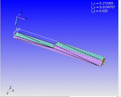
THe dimension of the geometry is 0.27*0.019*0.025

1.Material

after the formation of the geometry we take air as the flowing materia.

2.Boundary condtion

after setting materila now we assign the boundary condtion the left of the step is given as the inlet and the right face of the step is given as the outlet .and we apply the inlet the preesure 113255pa and the temparature of 300K and the spieces of air .and the outlet the pressure as 101325. and top face and bottom face we give as the wall .at the walls the velocity is going to be zeo hence we give no slip condtion.

3.Intial condtion

Spieces of air with masss fraction of O2 as 0.77 and the mass fraction of the N2 as 0.23 at 300k and at 101325pa.

4.Mesh sizes and embedding

the mesh sizes used are

case 1-dx = dy = dz =2e-3m

case2 -dx = dy = dz =1.5e-3m

case3 -dx = dy = dz =1.0e-3m

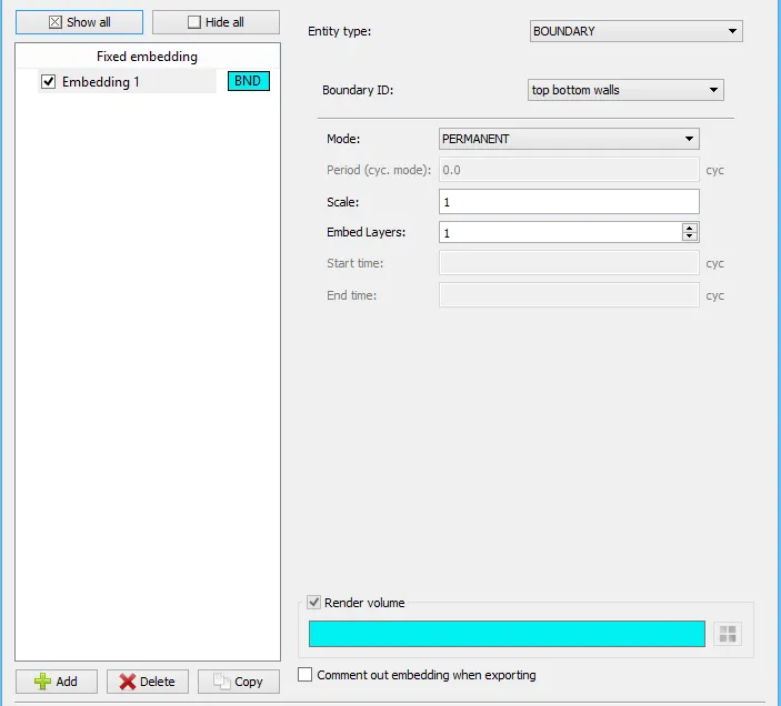
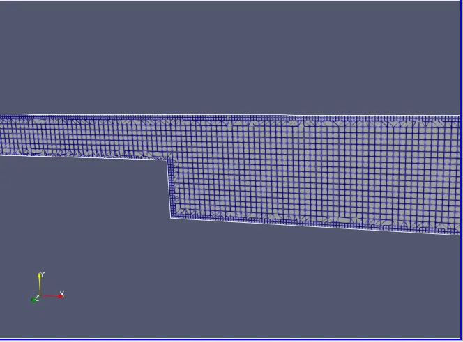
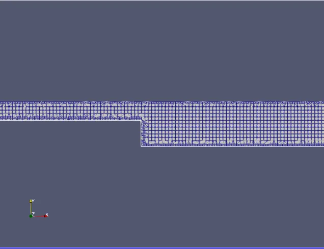
and we take check the fixed embedding and we get window like this and apply the embedding at the top and at bottom face as the boundary layer arond these faces is very thin and in order to encounter the velocity and the pressure becomes teadous hence we refine more at these regions hence to have better boundary layer.

5.Simulation and Time parameters

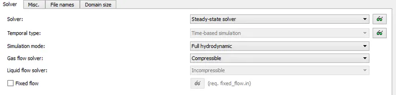
we use steady state solver with full hydrodynamic as there are no moving parts if moving parts involves the we have to select the transient solver.

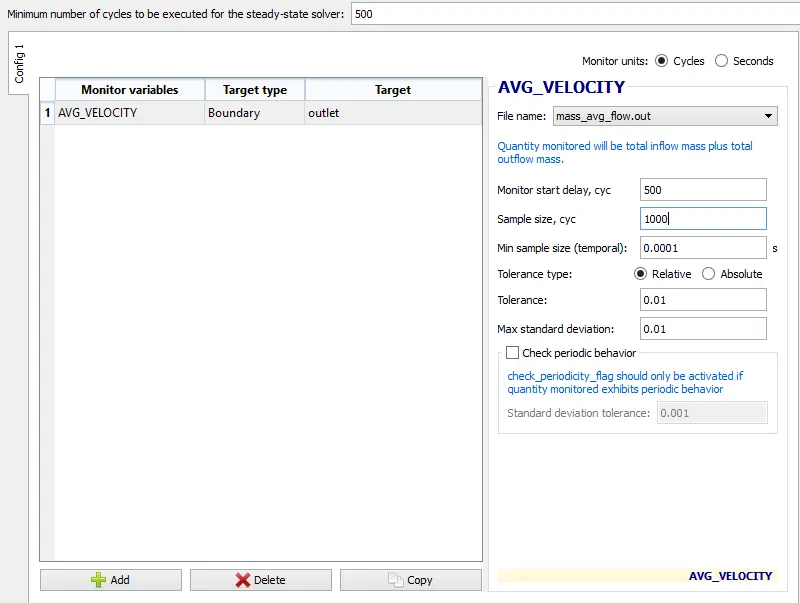
the time parameter are shown below

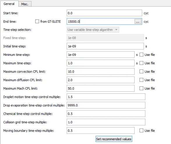
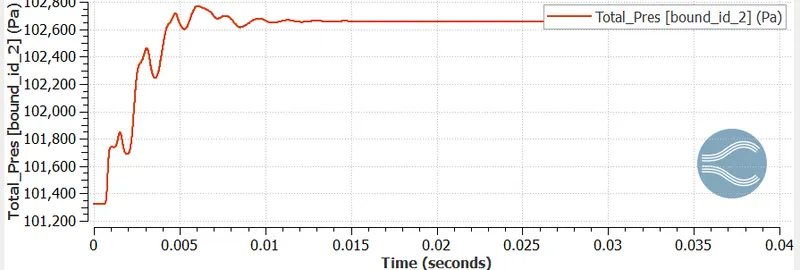
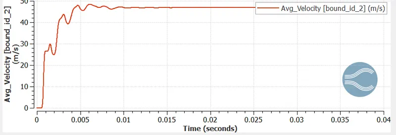
the simulation time starts from 0 cycles (here cycles for steady state and sec for transient solver)the end of the simulation depends on the solution attaing the convergence i.e the steady state starts monntoring for every cycles ande for every 1000 cycles it will check the tolerance of the average parameters for an example for 1000 cycles the average velocity is 2.25m/sec and for next 1000 cycles the average velocity is 2.24 and the tolerance bewteen the two cycles is 0.01 at this the simulation stops as it reached given tolerance if tolerance is not reched again its going to run but its going to run atleast minimum 500 cycles. and in the above plot the end time is taken apporixamately 15000 its not necessary for the simulation to run 15000 cycles.

6.post processing

The variables like the Temperature, pressure, velocity,Density,Turbulent viscocity and the Turblent KE are selected and time interval of writing 3d output files and text files are set such that 100 data files of each generated and the time interval for writing 3d output is 100s.

Export of input files

After setting the case set up in the coinverge now its to export the input files in the floder for the converge solver.

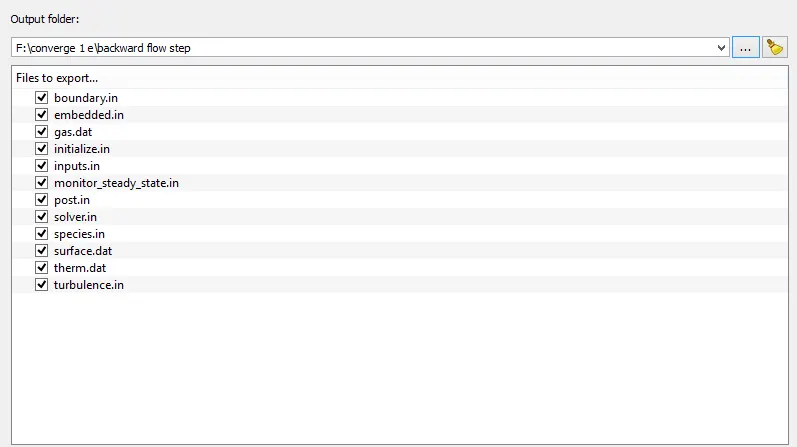
after the exporting files now its time to run the process. the process can be ruined in the window command plot or in the cygwin before running first we have to navigate in to the floder.for faster computional speed parallel processing is set up on 2 crores. The solver generates files #d output files and the .out files the out files contains information at the mesh points. and again 3d output files are further post processed using paraview tk binary format.

and we have the results for the case dx=dy=dz =1e-3

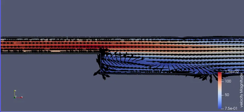
velocity contour for 1e-3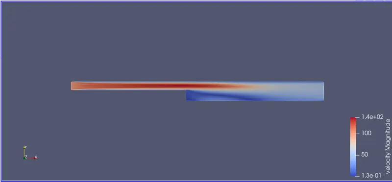

pressure contour for 1e-3

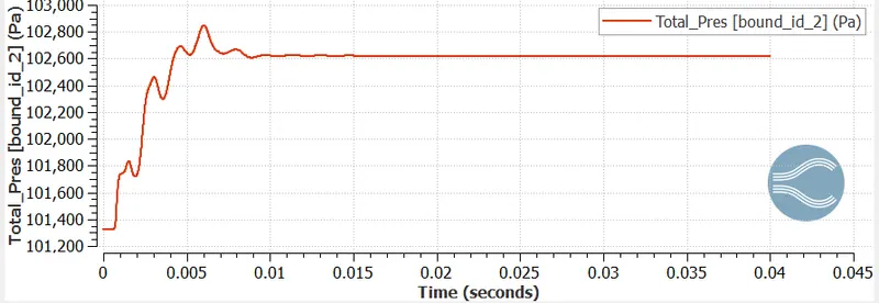
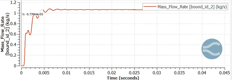
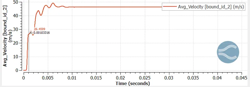
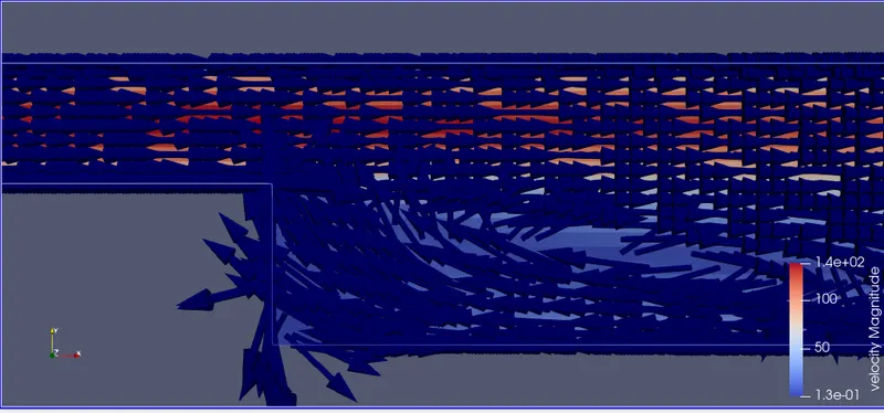
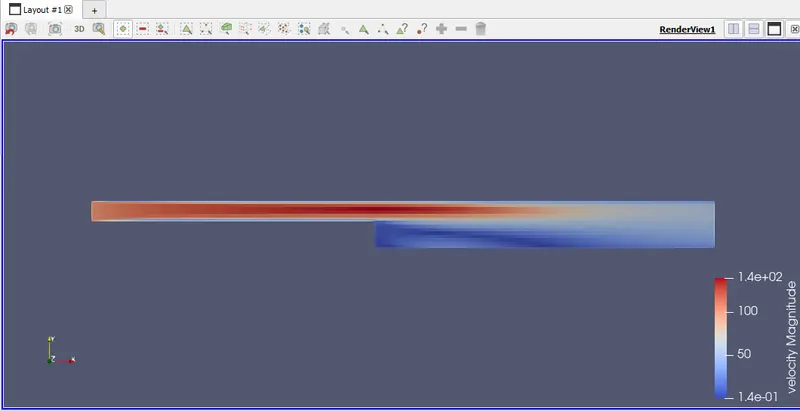
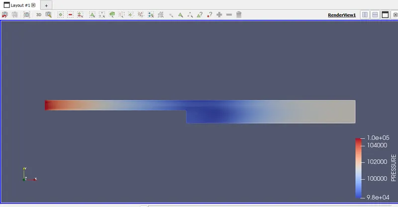
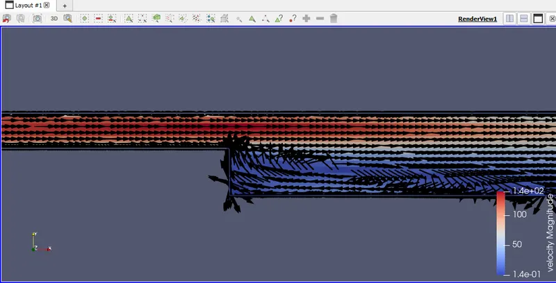
From above diagram we can observe the the boundary layer sepaertion had taken place as the area of the cross section increases the pressure gradient (dp/dx)will be greater than zero and hence the velocity gradient(du/dy) at that cross section is less than zeo and and the direction of the velocity reverses hence the bounday layer separtion take place due to which the recirculation take palce. at the other cross section the velocity gadient is greater than zero and the pressure gradient is less than zeo as the cross section is less

The results for 1.5 e-3

ve

velocity contour for 1.5e-3

pressure contour for 1.5 e-3

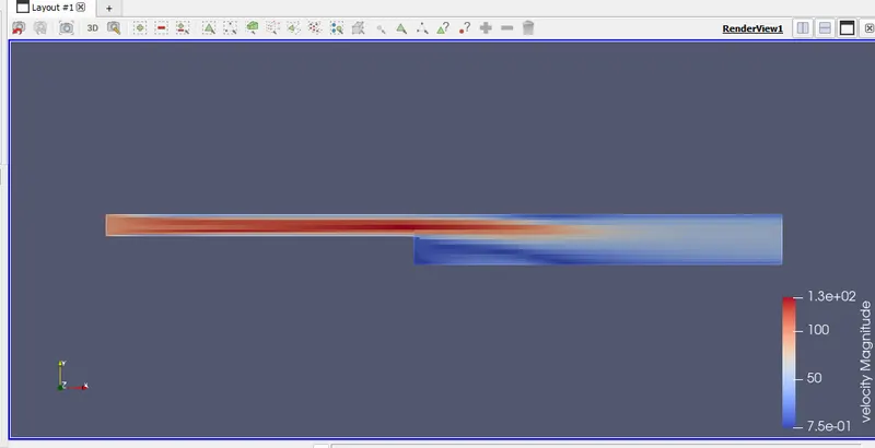
The results for 2e-3 is as follows

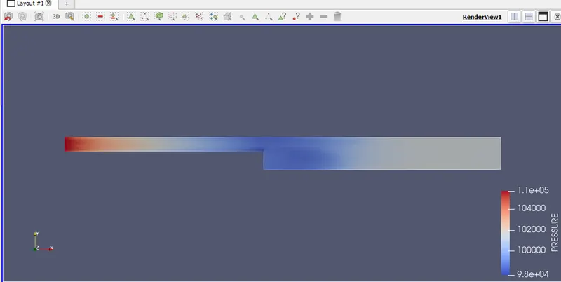
the pressure for 2e-3

Conclusion

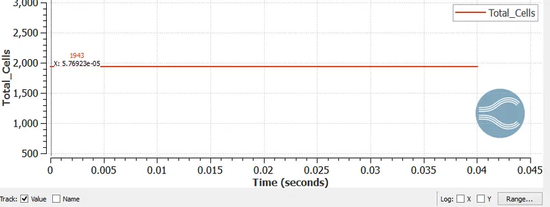
As mesh size decreases the cell count increases and the simulation time increases. and we can obseve that velocity increases at the inlet and velocity decreases at the outlet due to small cross section at the inlet and and at the outlat the velocity decreases and the pressure increases due to increases in the cross sectional area.and in all the casesv the mass flow rate almost same at the inlet.

sa

sa