Week 3: Flow over a backward facing step

Aim: to simulate the flow over a backward facing step using converge.

Objective: Run the case for three different base mesh sizes

1. dx=dy=dz=2.0e-3m
2. dx=dy=dz=1.5e-3m
3. dx=dy=dz=1.0e-3m

Case setup

1. import geometry in converge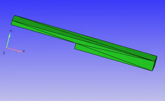

2. Assign triangles to a specified boundary

Inlet

outlet

Top bottom wall

Front_2d

back_2d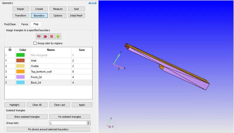

3. Run diagnosis and check for geometrical error.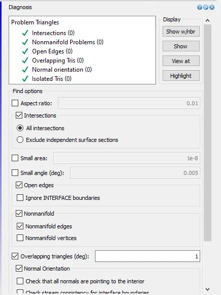

4. Begin case setup

• Application type
  time based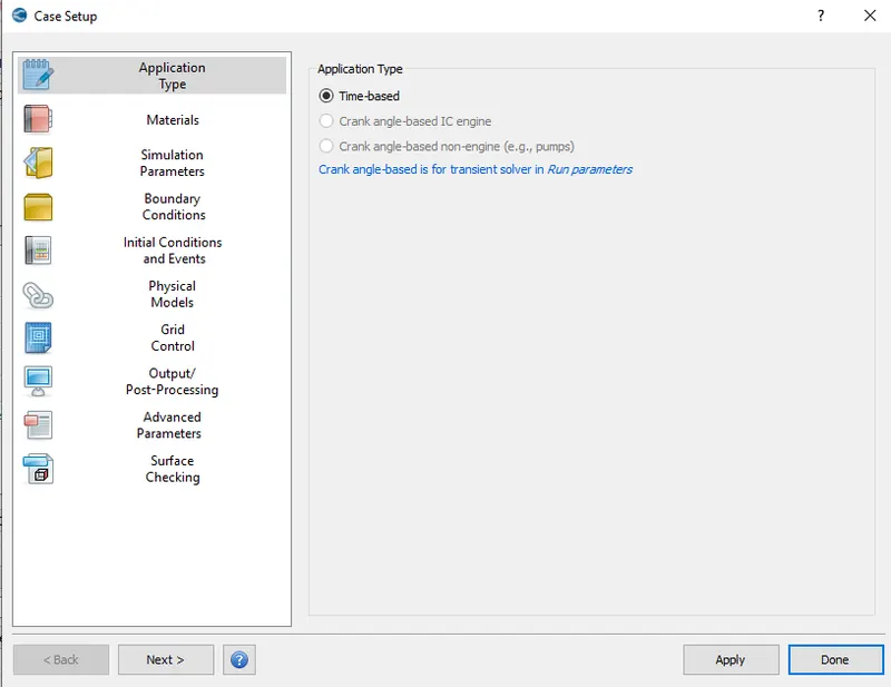
  
  
• Materials
  
  
  
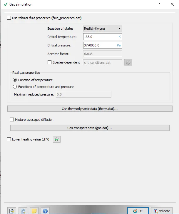
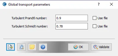
  Species
  `N_2` and `O_2`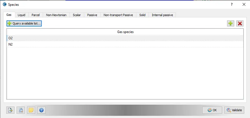
  
  
• Simulation parameters
  Run parameters
  Solver: steady state
  Simulation mode: Full hydrodynamic
  Gas flow solver: Compressible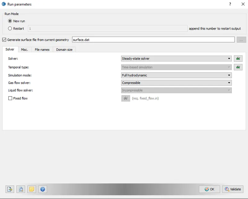
  
  Steady state monitor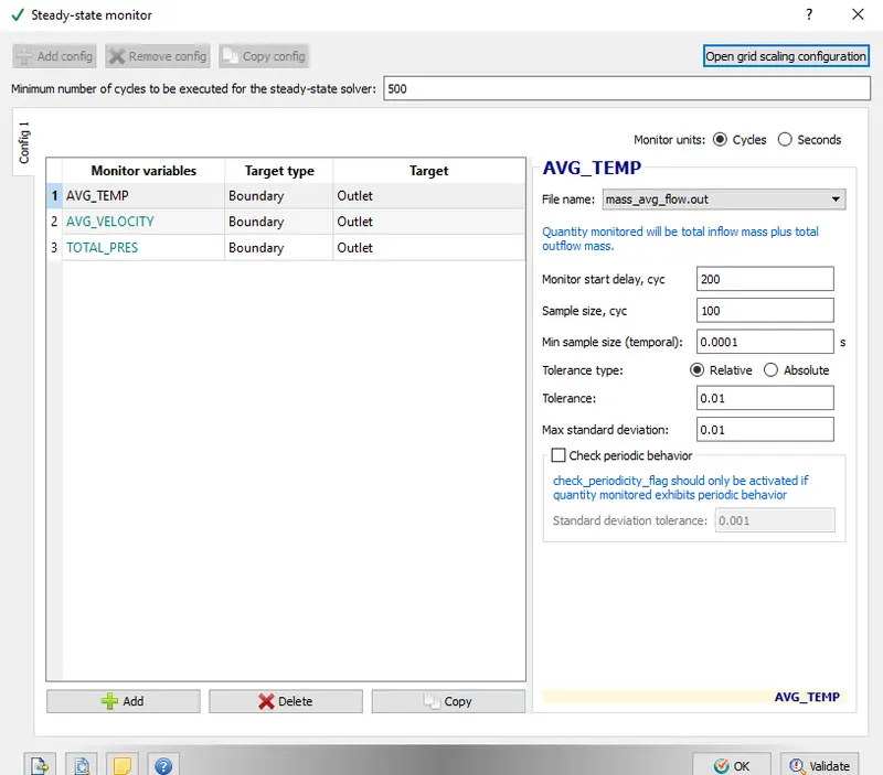
  
  Simulation time parameters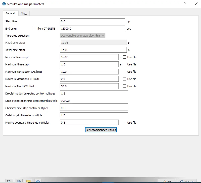
  
  Solver parameter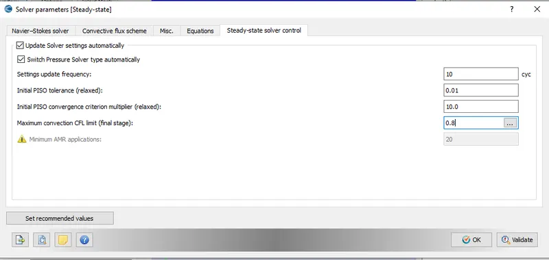
  
  
• Boundary conditions
  Inlet
  Boundary type: inflow
  Inlet pressure: 110325Pa
  Species: `N_2` and `O_2`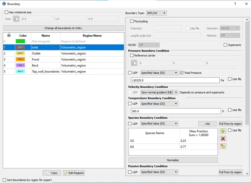
  
  
  Inlet
  Boundary type: outflow
  Inlet pressure: 101325Pa
  Species: `N_2` and `O_2`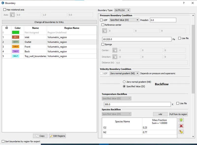
  
  Top wall Boundaries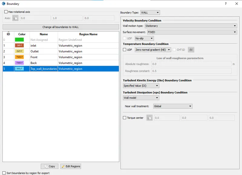
  
  Frond and back are of 2D Boundary type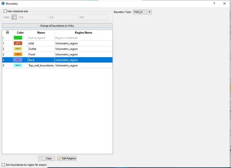
  
  
  
  
• Initial conditions and events
  Region name: volumetric region
  Temperature: 300K
  Pressure: 101325Pa
  Species: `O_2` and `N_2`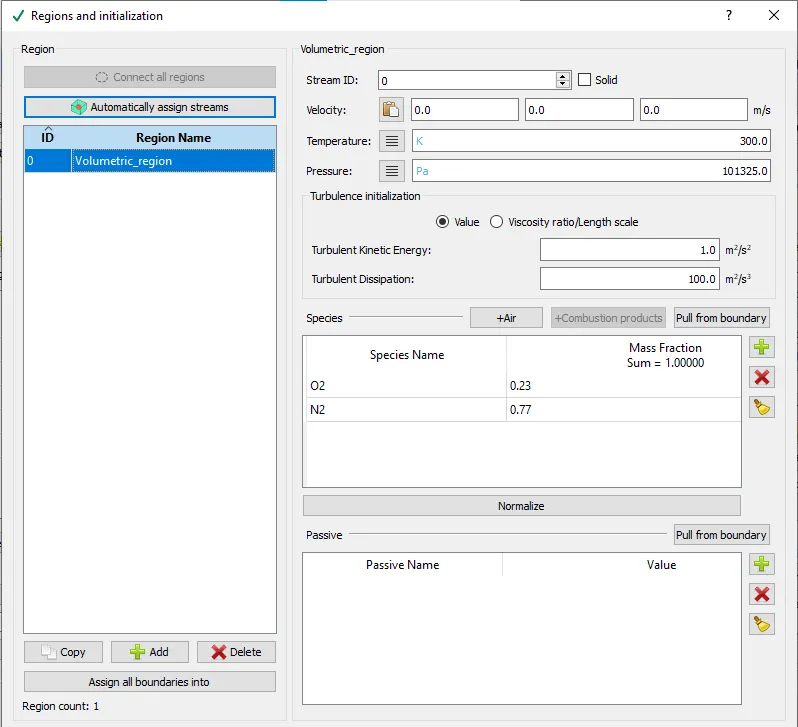
  
  
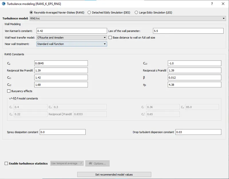
• Turbulence model
  
  
  
• Grid control
  here we can set any grid size as per requirement and computer capacity.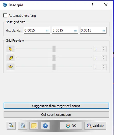
  
  
  
• Post variable selection
  here we can choose variables from the list of the variables to post process the result.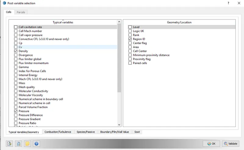
  
  
  
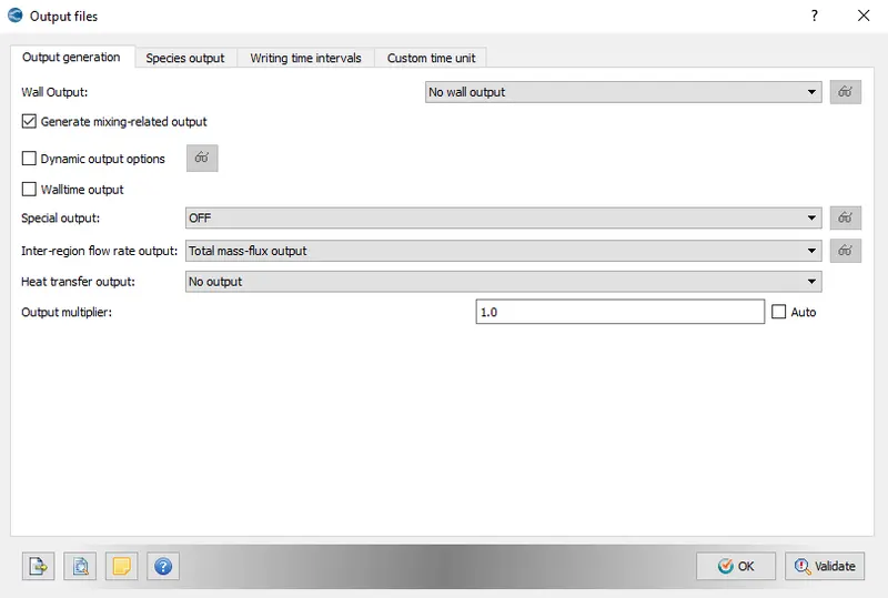
• Output files
  
  
  
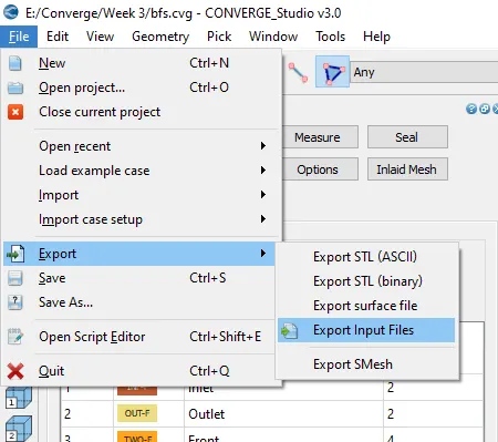
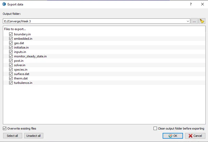
• Export input files
  
  
  
  
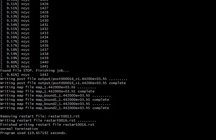
• Run the case setup in Cygwin
  
  
  
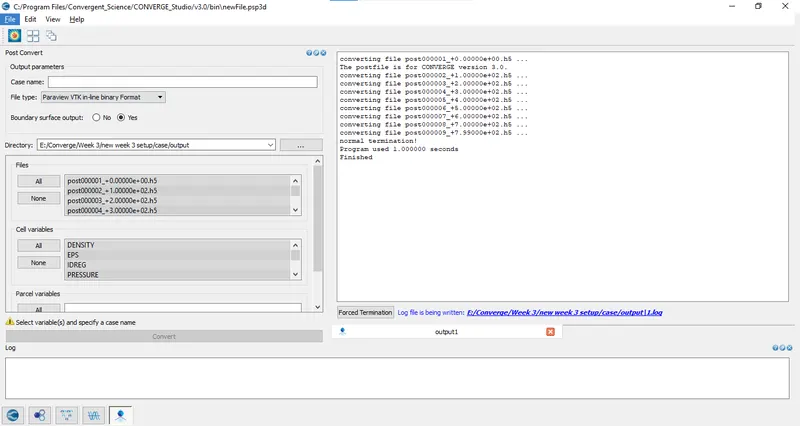
• Convert the out file in .vtm format
  
  
  

Recirculation region

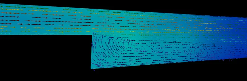
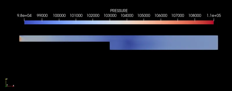
Due to the break is causing the fluid to create recirculate zones which are better termed as eddies. From the above snapshot it can be observed that there is turbulence near the dam break which is signified by the blue colored low-pressure zone. Then the diffusion takes place as the least pressure zones become shorter and moves forward with the flow. After that we can see as it moves forward there are trailing vortices which are formed behind the mother vortices which is the least pressure zone.

Output for case 1e-4
Mesh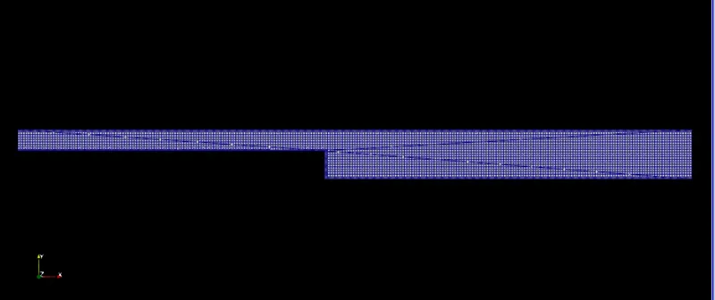

Cycle vs Pressure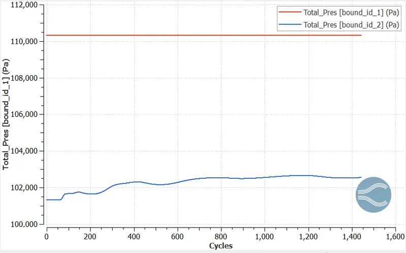

Cycle vs velocity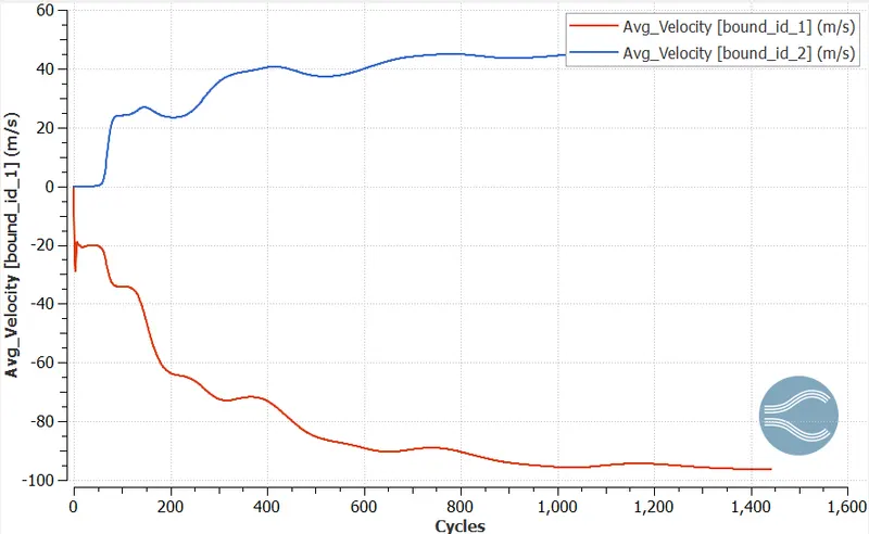

Average velocity at inlet = -95m/s and at outlet 45m/s
Mass flow rate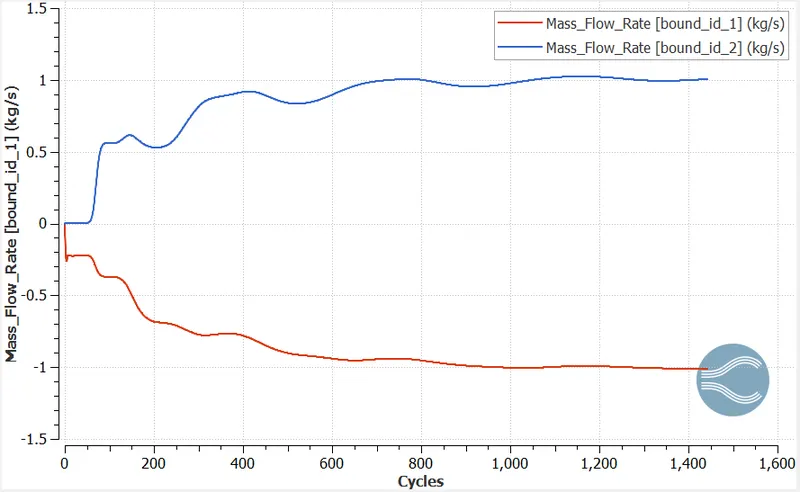

mass flow rate at inlet = -1kg/s and at outlet 1kg/s

Cell count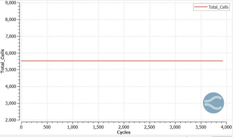


Output for case 1.5e-4

Mesh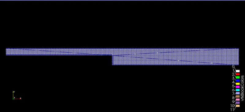

Pressure plot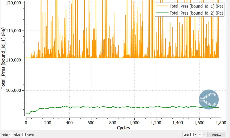

Velocity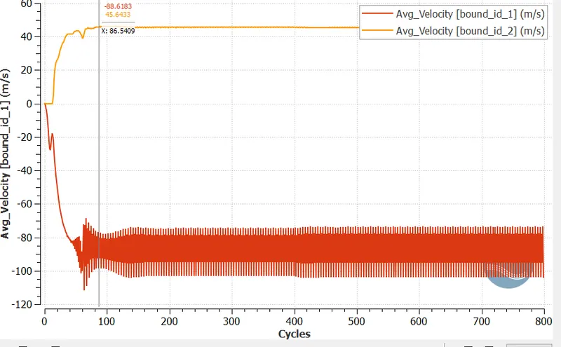

average velocity at inlet is approximately -90m/s and at outlet 45m/s.

mass flow rate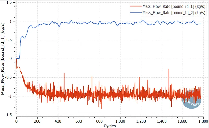

mass flow rate at inlet is approximately -1kg/s and at outlet 0.8kg/s

Cell count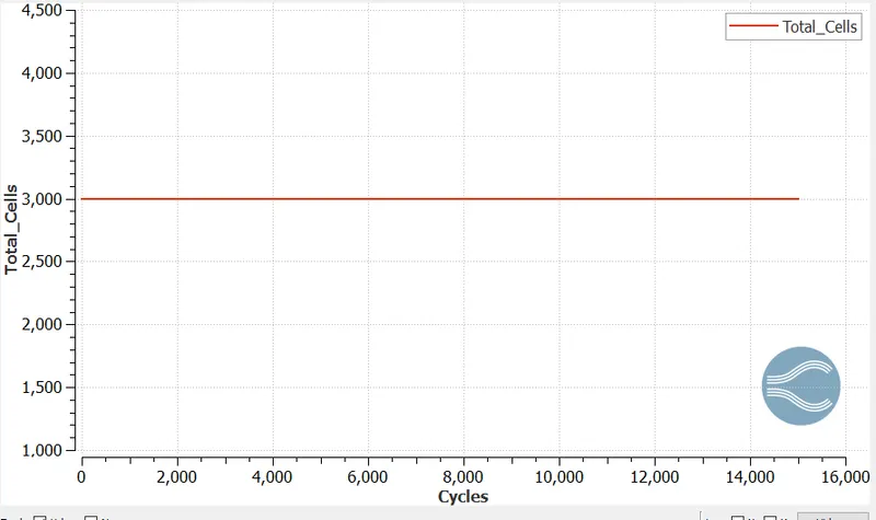

Output for case 2e-4

Mesh

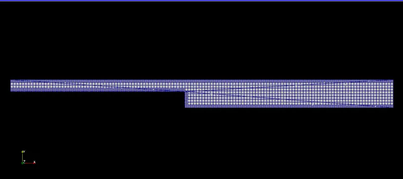
Pressure plot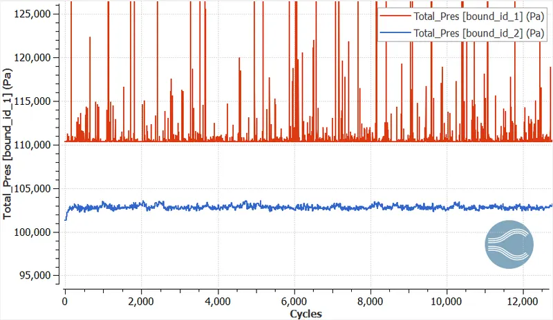

Velocity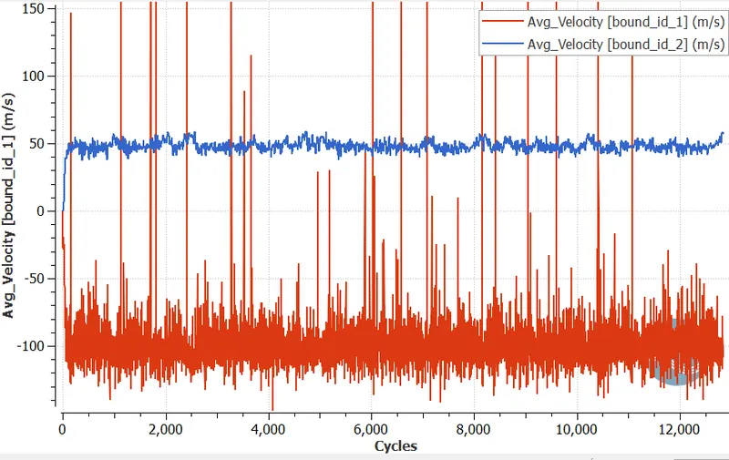

Average velocity at inlet is approximately -100m/s and at outlet 50m/s

Mass flow rate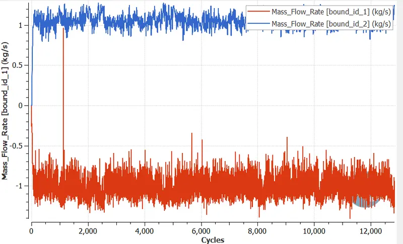

mass flow rate at inlet is approximately -1kg/s and at outlet 1kg/s

Cell count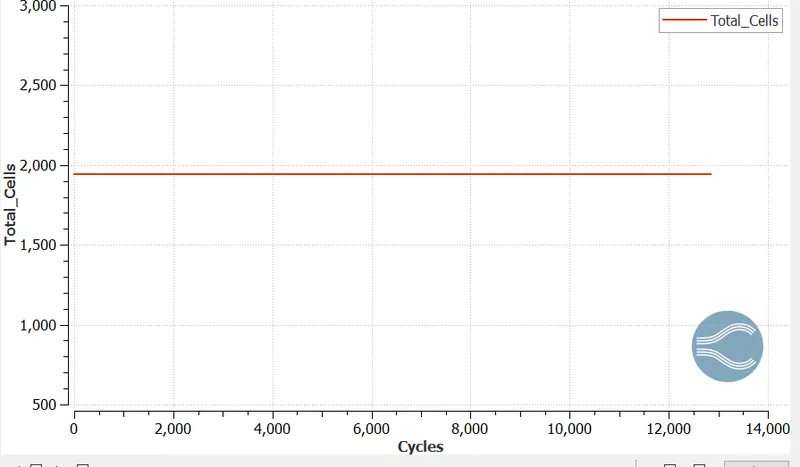

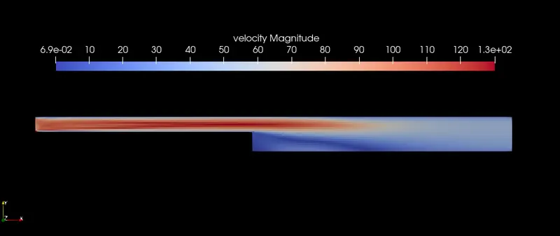
Velocity contour

Pressure contour

Velocity Contour animation link

https://youtu.be/uLSzhUfI4ls

Velocity Contour animation link

https://youtu.be/CZi6QrvvcbY

Conclusion

• As we increase the grid size computational time increases.
• in all the cases we can see mass flow rate is conserved.
• The average velocity at the inlet is higher than that of outlet because of sudden expansion region.