Week 3: Flow over a backward facing step
- Aim - Flow over a backward facing step
- Objective - To Simulate the flow of air over Backward facing step.
- The case should be run with 3 different mesh sizes
- Post processing of the flow parameters
- dx = dy = dz =2e-3 m
- dx = dy = dz =1.5e-3 m
- dx = dy = dz =1.0e-3 m
- Backward facing step
- Backward-Facing Step (BFS) flows include aerodynamic flows (wings, spoilers, high angle-of-attack processes), engine flows, condensers, vehicles (cars, boats), heat transfer systems, and even flows around buildings.
- Flow separation after the simple phase leads to the formation, development and reattachment process of separated bubbles. This depends on the geometrical design of the BFS, inlet and outlet conditions, and turbulence intensity as heat transfer conditions.
- It has been extensively studied in the last decades by various theoretical, experimental and numerical methods.
- Various applications of BFS flow can be found in our daily life, such as flow in engine inlet tunnels, flow in condensers/combustors, and flow around boats and buildings (or structures).
- Spreading flow, countercurrent, diverging flow path or countercurrent includes the basic characteristics of general separation flow. This is inherently 3D, which lends itself to his 2D discussion for certain flow conditions and simple step geometries. This is an important model for separated flows over a wide range of Reynolds numbers.
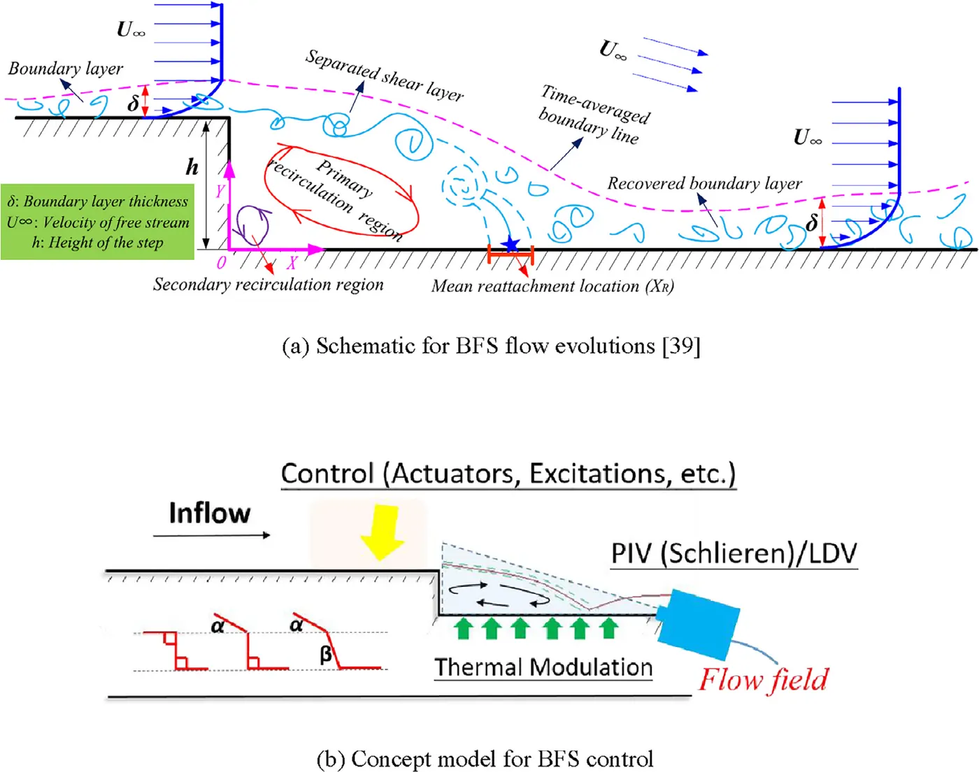
- Backward stepping (BFS) flow, also known as ``fast-scaling flow'', ``circular-scaling flow'', ``backward flow'', ``divergence channel'' or ``backward flow'', constitutes a common fundamental feature. Separation flow. This is inherently 3D, which lends itself to his 2D discussion for certain flow conditions and simple step geometries.
- Procedure
- Geometry
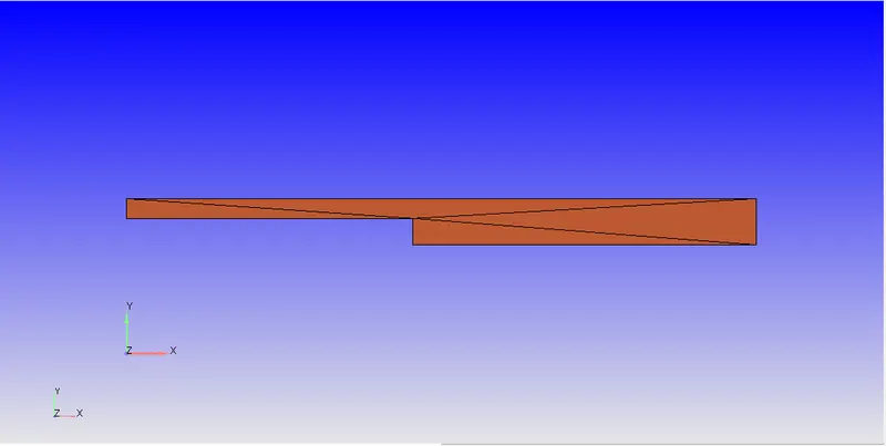
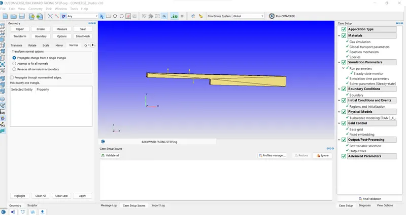
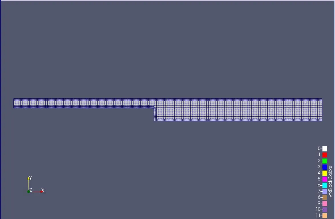
- Mesh
- Setup
-
Now for the mesh we have taken the mesh size of
dx = 2e-3m
dy = 2e-3m
dz = 2e-3m
BOUNDARY CONDITIONS
Inlet Boundary
- INFLOW BOUNDARY
- Pressure = 110325 Pa
- Mixture - Air
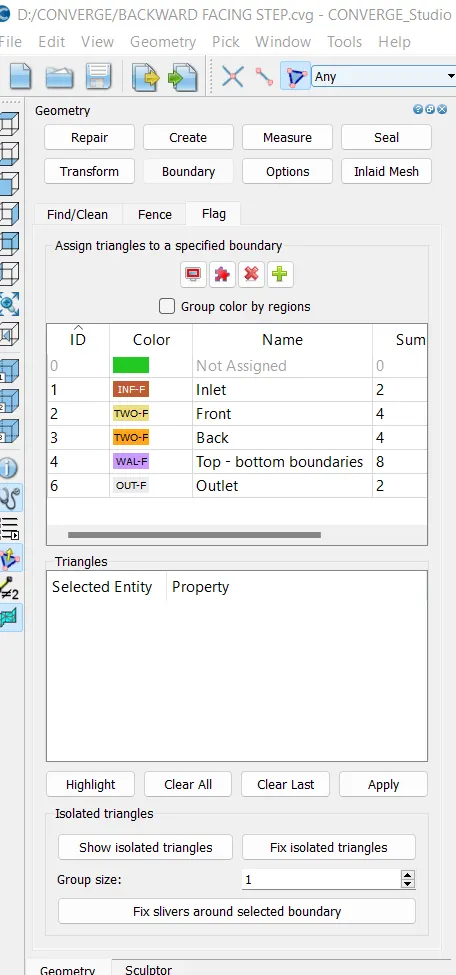
Outlet Boundary
- OUTFLOW BOUNDARY
- Pressure = 101325 Pa
- Mixture - air
Top and Bottom Walls
- WALL BOUNDARY
- Temperature = 300 K
- Velocity - Stationary
- Temperature - Law of Wall
- Turbulent Kinetic Energy - Zero normal gradient
- Turbulent Dissipation - Wall model
- Results
- Grid size
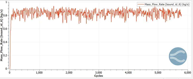
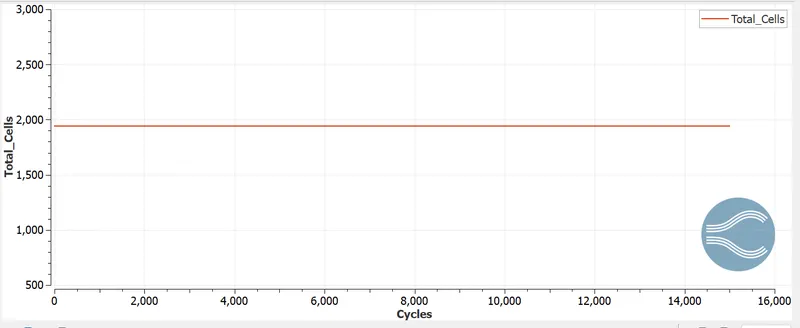
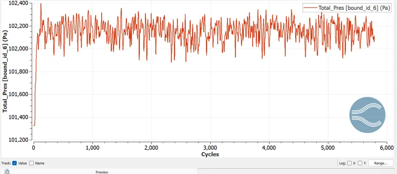
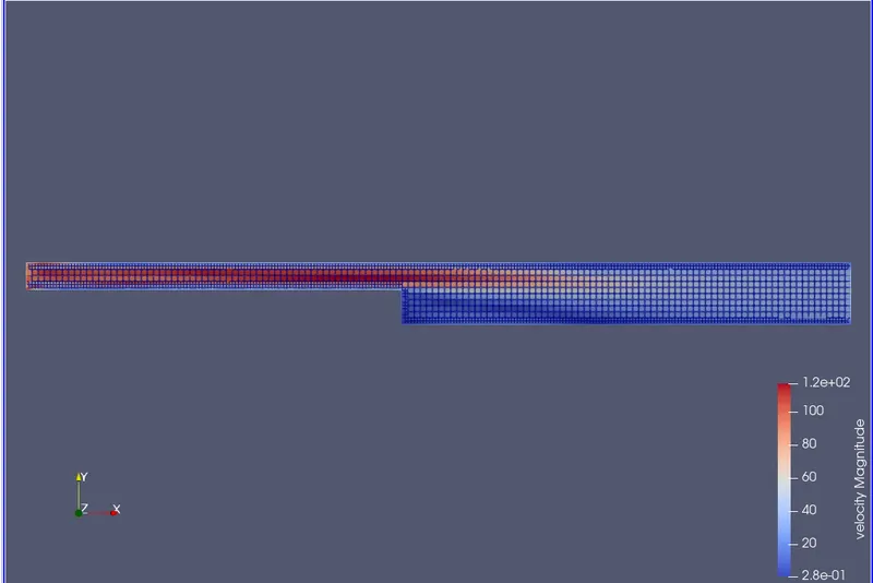
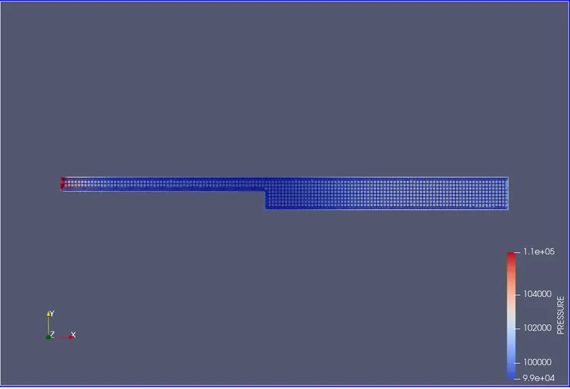
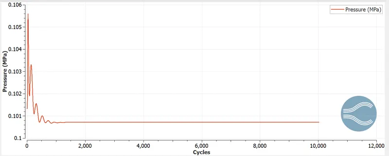
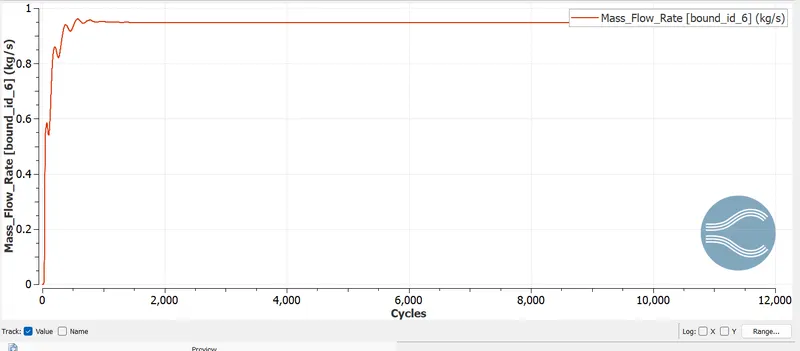
- dx = dy = dz =2e-3 m
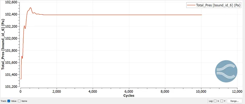
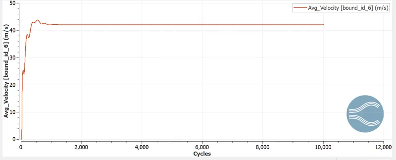
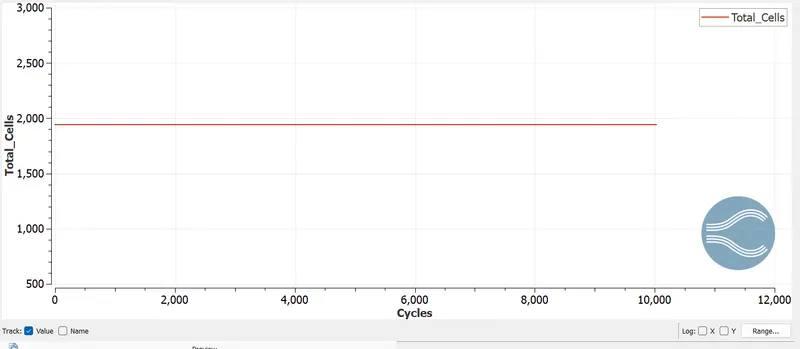
- Grid size
- dx = dy = dz =1.5e-3 m
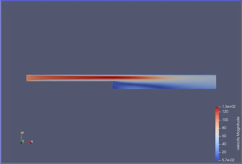
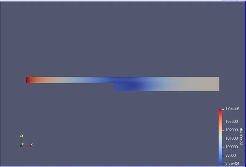
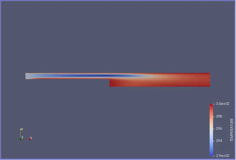
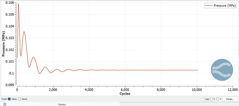
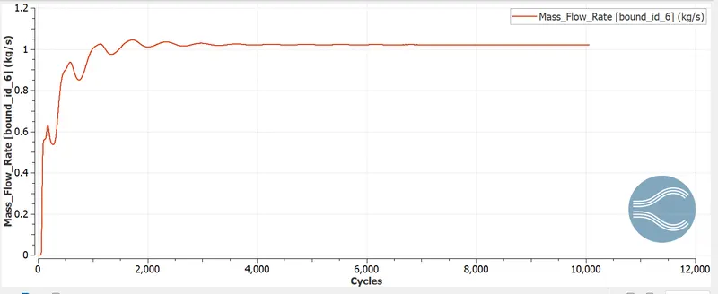
- Grid Size
- dx = dy = dz =1.0e-3 m (If this is too much for your PC, use 1.2e-3 m)
- 1.2e-3
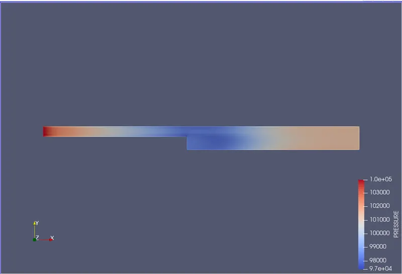
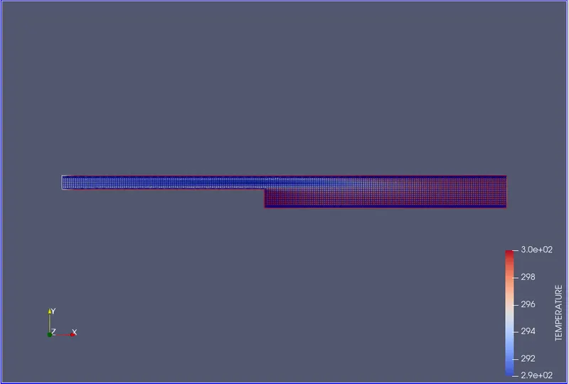
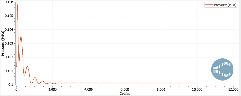
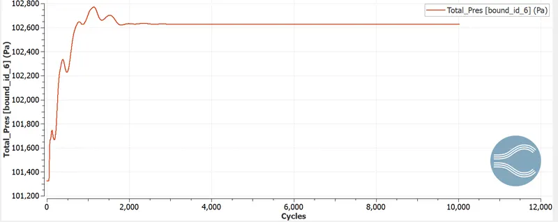
- Google Drive link for animation.
- Link-https://drive.google.com/drive/folders/12qXouHtxU0CyvnaLtIiL4p451C6sTJXW
- Stepwise Explaination
- Peprocess:Open CONVERGE Studio. Import and load .stl files (geometry models).
- Specify the extents of the geometry.
Simulation Setup:To run the simulation, select Time-based as the Application Type. Click Apply and Done. Check "Gas - Simulation" and "Species" and select the "Air" material as the defined mixture.
- For the global transport parameters, we write the turbulent Prandtl number as 0.9 and the turbulent Schmidt number as 0.78. Click OK and Validate. For seeds, click the "plus" icon to add a new seed.
- Since this simulation is a gas simulation, let's add N2 and O2 to the Gas tab. For the Solver tab run parameters, specify Solver as Steady State Solver, Simulation Mode as Full Fluid Dynamics, and Gas Flow Solver as Compressible.
- For Steady-state solver parameters, use the Navier-Stokes density basis. Solver - type On the Equations tab, ensure that the preconditions for all equations are set to None.
- Create a steady-state monitor for Avg. speed. A speed monitor is a setup with a tolerance to observe the convergence of results. Once the simulation setup is complete, export the input files to the desired folder.
- Click File and click Export. Select the Export Input File option.
- Select a folder to export the input files and click OK to complete the process. To run the simulation, open a Cygwin terminal and open the folder containing the input files.
- Run the command "mpiexec.exe -n 4 convert.exe limited logfile &". Add mpiexec.exe to converge before running the command.
- Observation
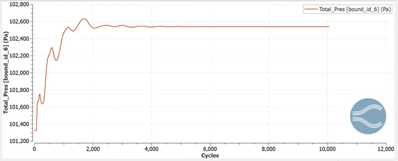
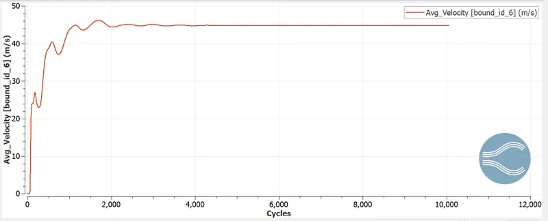
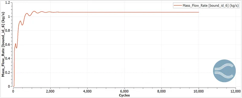
- It can be seen that the mass flow rate is more or less conserved in all three cases.
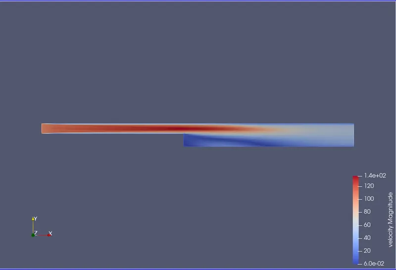
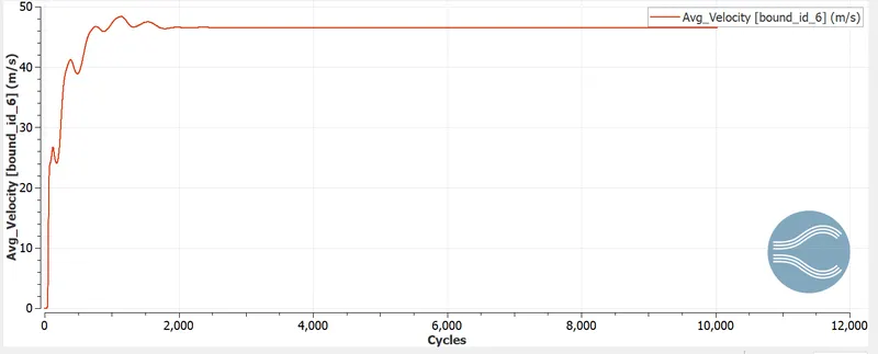
- The average inlet velocity we find is higher than the outlet, which must be due to boundary layer separation or recirculation zones created in regions of rapid expansion. This is due to the loss of kinetic energy in the B.L separation.
- The static pressure drops in the recirculation area.
- Static pressure is constant at the outlet and decreases at the inlet limit, total pressure is constant at the inlet and increases at the outlet.
- The static pressure is higher at the exit boundary than at the entrance, evident because the altitude is higher than the entrance.
- Similarly, the absolute value of the total pressure at the outlet will be lower than the pressure at the inlet due to small changes in pressure from left to right.
- The total pressure drop at the outlet dictates the direction of flow from left to right.
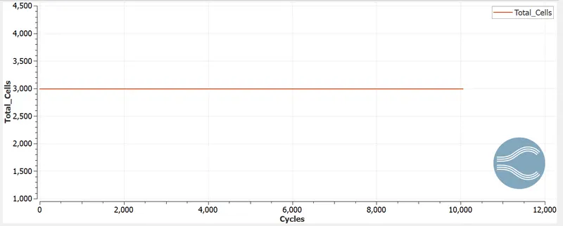
- The number of cycles each mesh goes through is based on the initial temporality of the problem and the mesh size and tolerance limits. As can be seen from the figure, the first transition settles down once steady state is reached and the simulation stops.
- Conclusions
- Simulations were performed with three different mesh sizes.
- flow variables were plotted against cycle number.
- Contour plots show the distribution of the flow variables .
- In vector plots, recirculation zones can be observed near the steps.
- Static pressure drops due to motion losses in the boundary layer region.
- Small deviations in values such as mass flow rate, average velocity, etc. can be seen during the simulation.
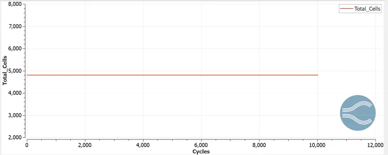
- Increasing the number of cells increases solution accuracy and simulation time. Detailed turbulence can be observed from the velocity vector contours as the mesh side becomes smaller.