Week 3: Flow over a backward facing step

AIM:

To simulate the flow of air through a backward facing step using converge CFD.

OBJECTIVE:

• To setup and run the simulation for three different grid sizes and compare the results.
• To plot velocity contour, pressure contour, mass flow rate and total cell count for all the 3 base mesh sizes.

INTRODUCTION:

BACKWARD FACING STEP:

Backward Facing Step (BFS) is widely known for its application in the studies on turbulence in internal flows. The flow separation is caused due to the sudden changes in the geometry. This creates a zone of re-circulation and a point of flow reattachment.

 

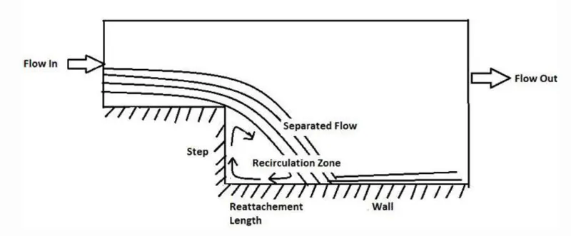
Fully developed flow enters the domain from left. When the flow reaches the step, because of expansion of flow channel, pressure gradient exists, it detaches and a recirculation zone is formed. A turbulent boundary layer encounters a sudden back step, causing flow separation. Later the flow eventually reattaches to the bottom wall.

CASE SETUP:

• Geometry is imported to the workspace from the stl file given above.

                     

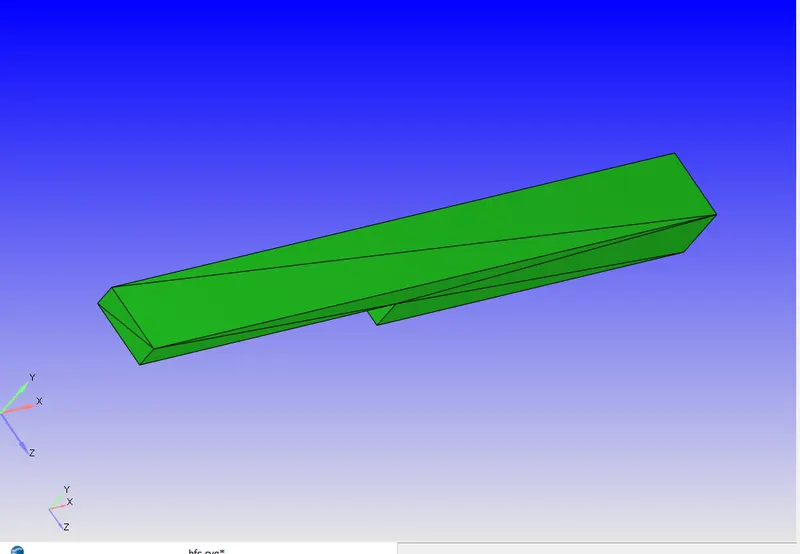
• The boundary are created for the geometry under boundary flag tab.

         

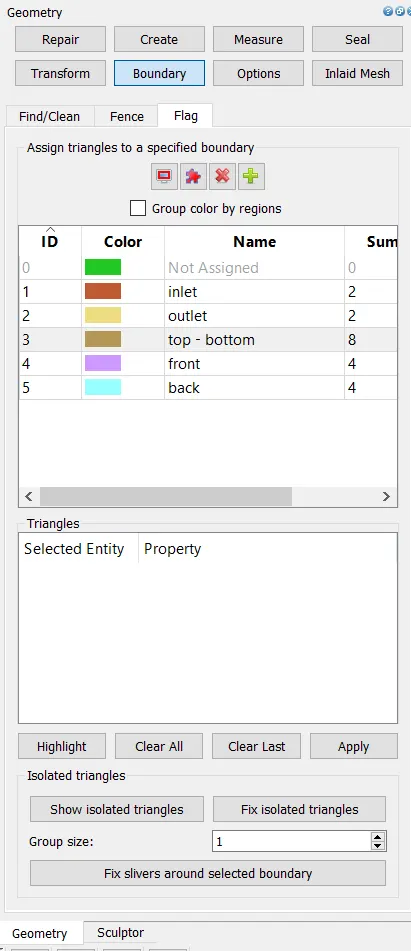
         The boundaries are assigned to the faces and the name of the boundaries are edited and click apply.

• The orientation of normal are checked and its changed such that the normal points inwards by going to transform > normal

        

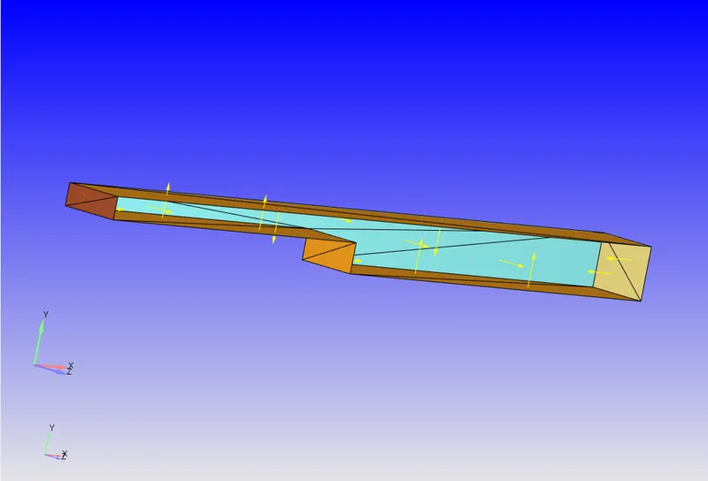
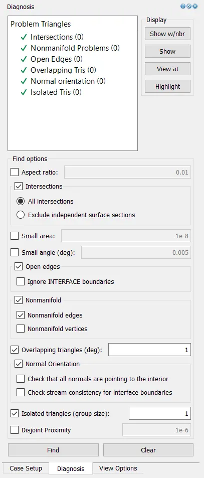
• The diagnosis is runed and checked for problems for the geometry.

         

• Begin case setup:
• Application type

        On the right panel go to the case setup tab, select begin case setup.

         

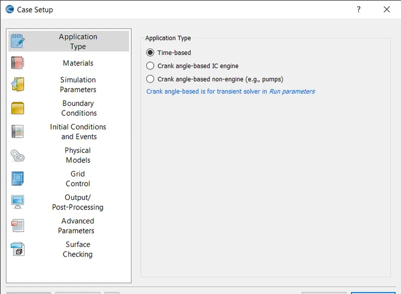
         Select the application type as time-based and select apply and done.

• Materials

        Select materials and select the checkbox reaction mechanism then select the predefined mixture as air then click apply and done.

• Gas simulation

         

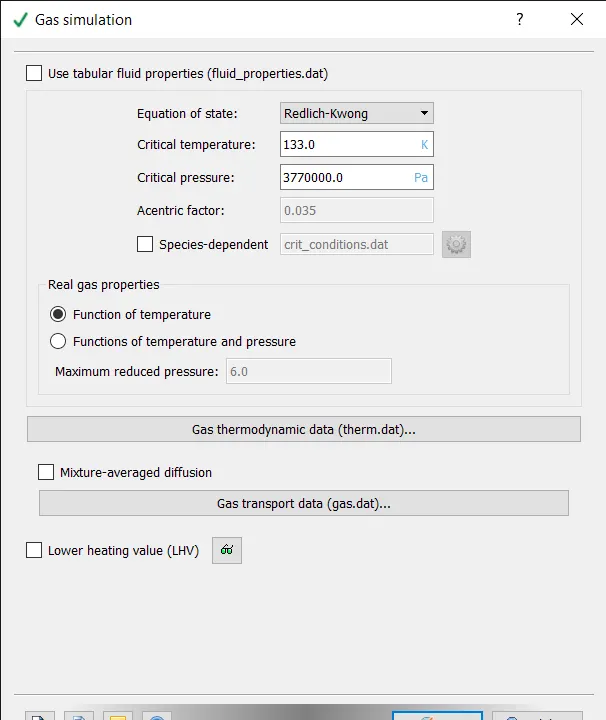
         The default values are selected and press ok.

• Global transport properties

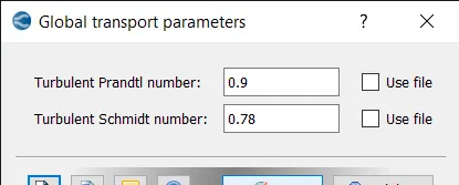
        Select global transport properties, keep the default values and press ok.

         

• Reaction Mechanism

        

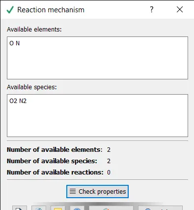
        The reaction mechanism are left default and the species are checked by using check properties.

• Run parameters

        Under solver tab select solver as steady-state solver

        

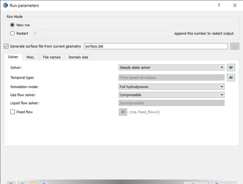
        Under misc. tab enable steady-state monitor and disable the used shared memory.

• Simulation time parameters

        

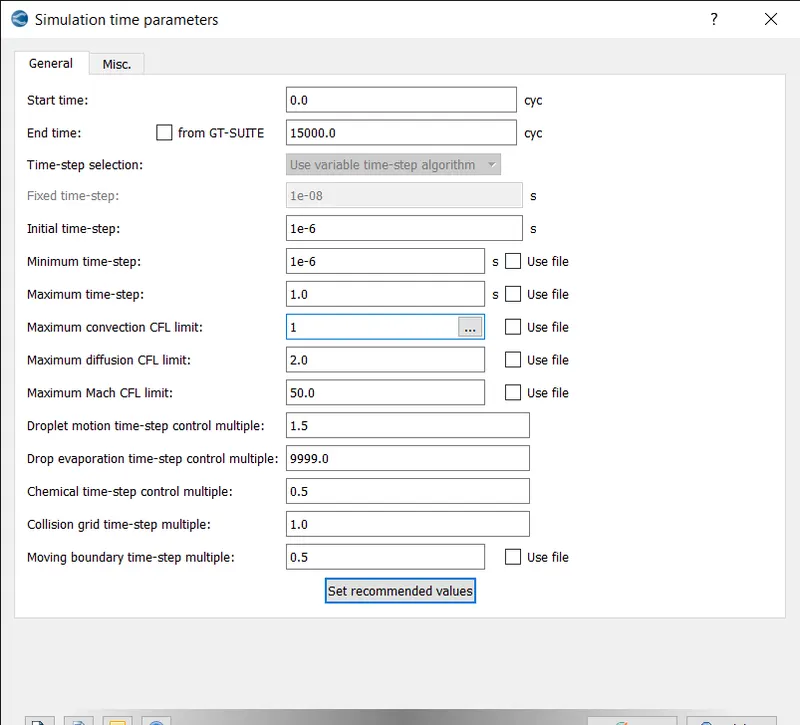
        Set the start time, end time, initial, minimum and maximum time steps as shown above.

• Solver parameters

         

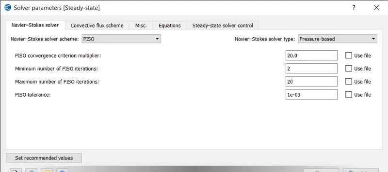
         Select the navier-stokes solver type as pressure based and click ok.

• Regions and initializations

         

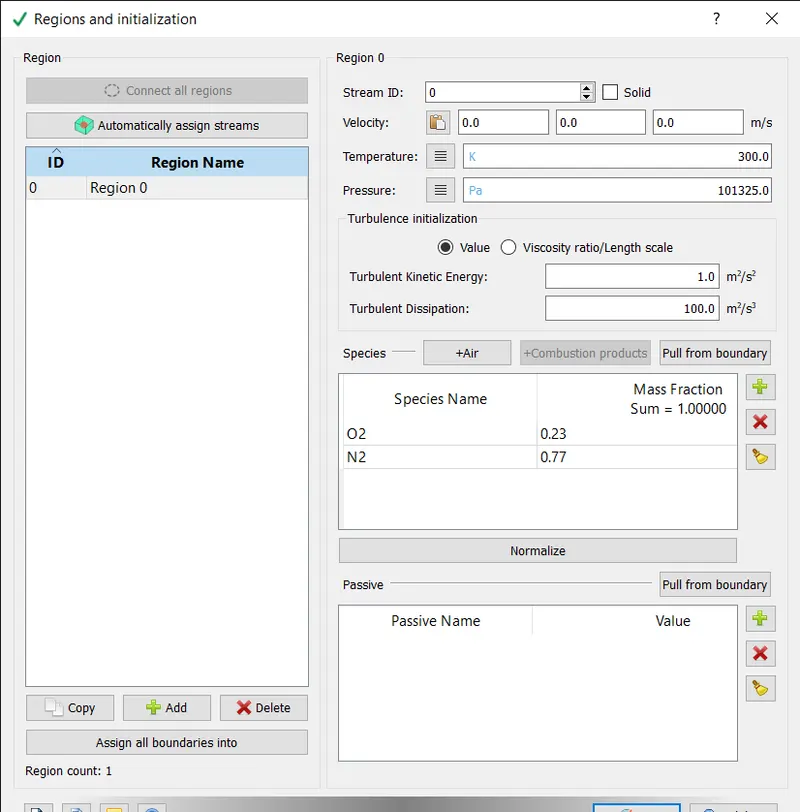
         The regions are created and air is added as species and mass fractions are changed to O2 as 0.23 and N2 as 0.77.

• Boundary conditions

        Inlet:

         

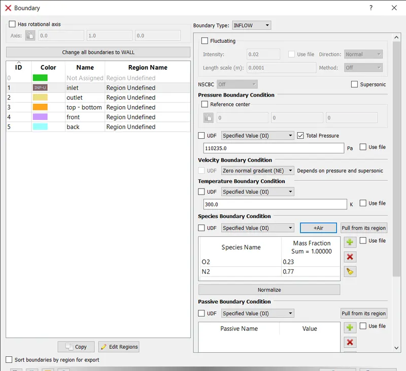
         For inlet, set the pressure boundary condition as specified value of 100001 pa and select air for species boundary conditions.

         Outlet:

          

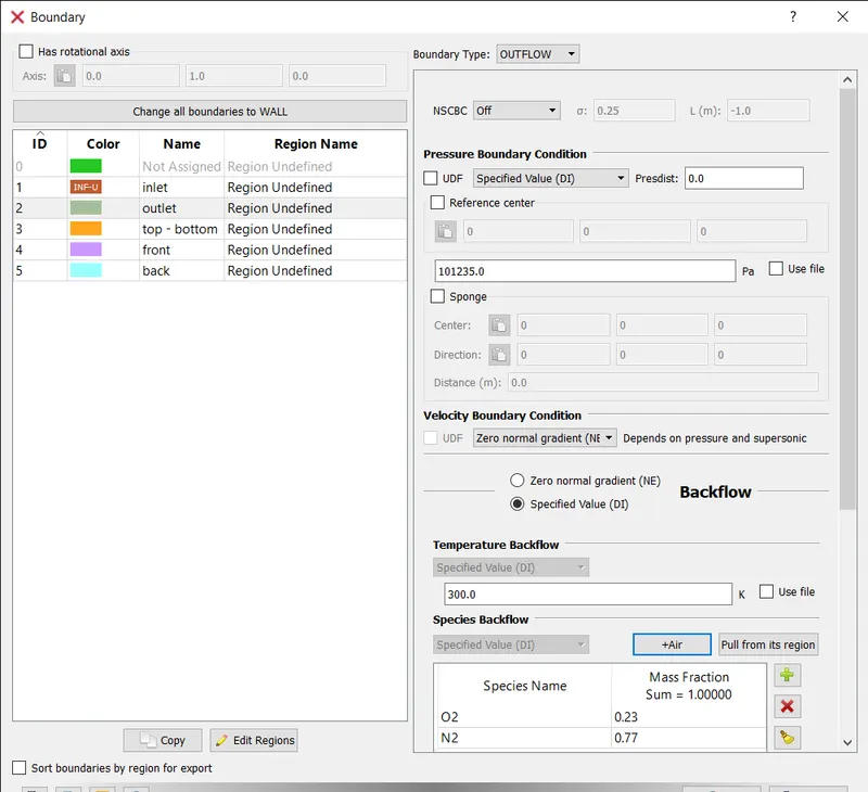
          Set the outlet pressure boundary conditions as specified value of 100000 pa and for species backflow select air.

         Top and bottom:

          

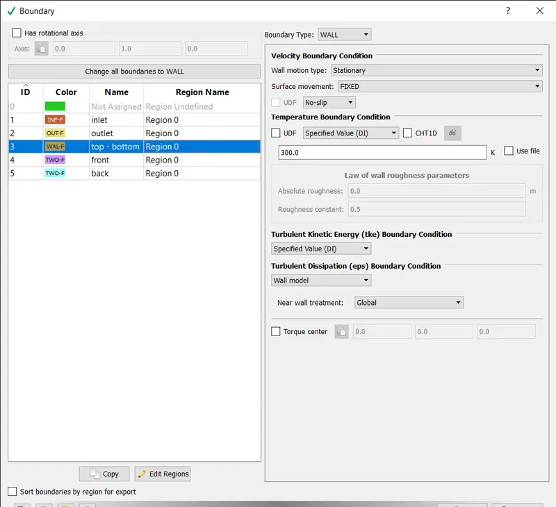
          Select the top and bottom boundary as wall type with no slip boundary conditions. And the temperature as specified values of 300k.

          Front and back:

           

           

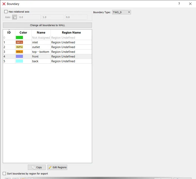
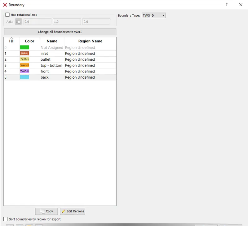
          The boundary type is selected as 2d.

• Steady state monitor

         

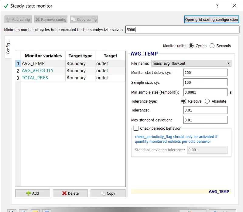
          The monitor variables are added and the minimum number of cycles, monitor start delay and sample sizes are defined.

• physical model

        

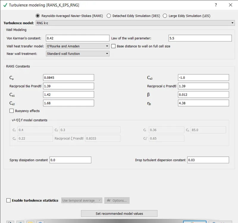
        The default values are selected and click ok.

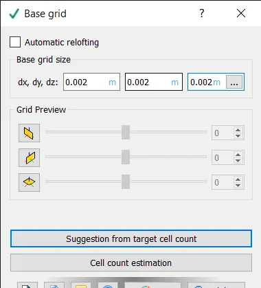
• Base grid

         The three different base grids are defined for three different cases and press ok.

          

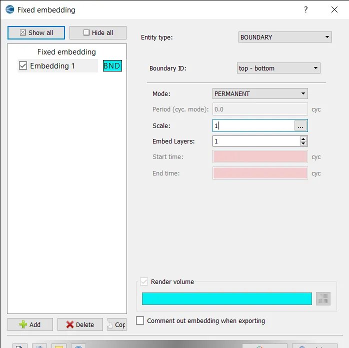
• Fixed embedding

        

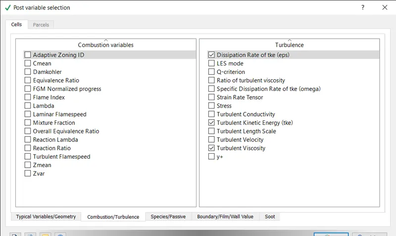
• Post variable selection

         

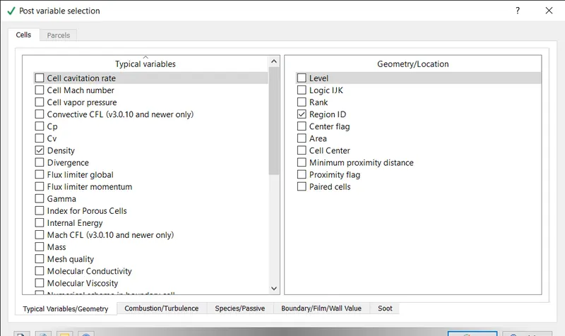
         Keep the default values in typical variables tab.

          

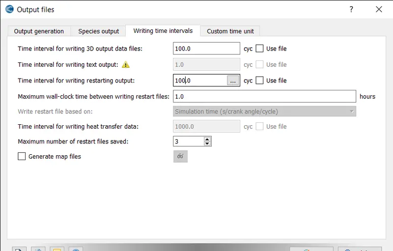
• Output files

         The interval for writing 3d output data files and restarting outputs are defined.

          

• Exporting the input files to a folder
• Then the executable is pasted inside the folder
• The simulation is run in Cygwin for three different base mesh grid sizes.
• The postconvert executable is pasted in the output folder.
• The post conversion is done on Cygwin and converted into the type that paraview reads.
• The results are then post processed using paraview.

RESULTS:

CASE 1:

MESH: (2e-3 m)

 

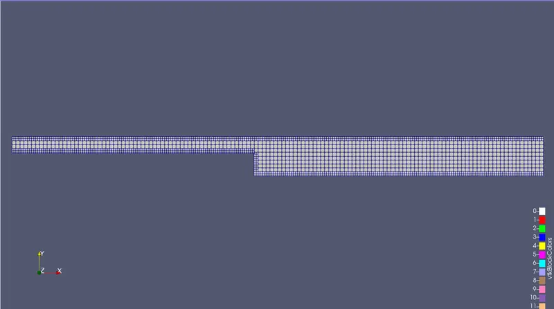
VELOCITY CONTOUR:

 

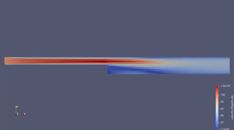
From the above plot we can say that velocity is high where the cross sectional area is less and velocity is less in the recirculation region.

PRESSURE CONTOUR:

 

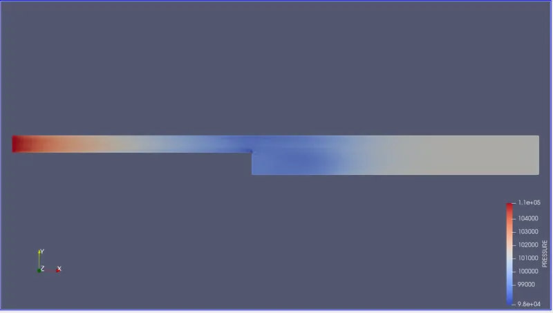
From the above plot, the pressure is less near the step or flow separation region. 

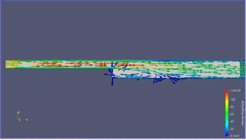
GLYPH:

VELOCITY PROFILE:

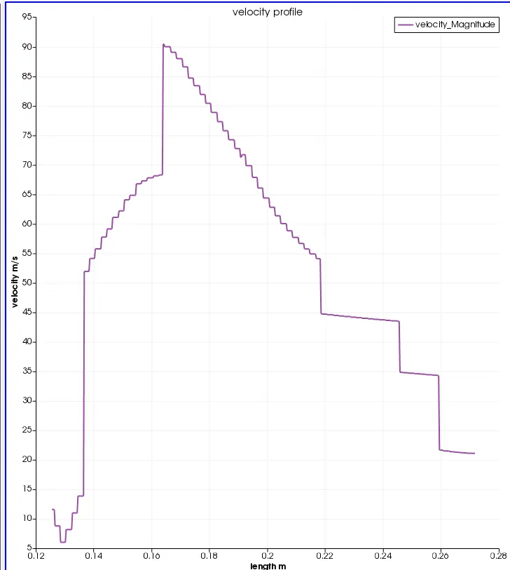
From this plot, the velocity increases near the step and then decreases.

PRESSURE PROFILE:

 

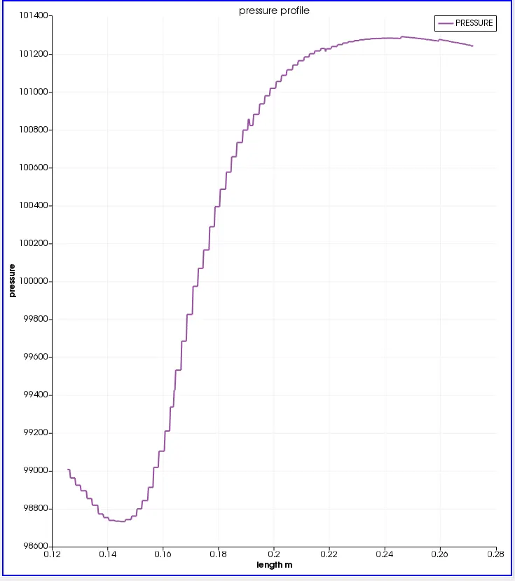
From this plot, we infer that pressure decreases near the step and then again increases.

CELL COUNT:

 

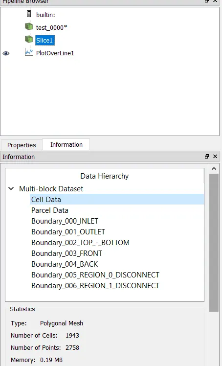
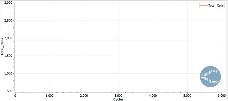
Number of cell count is 1943.

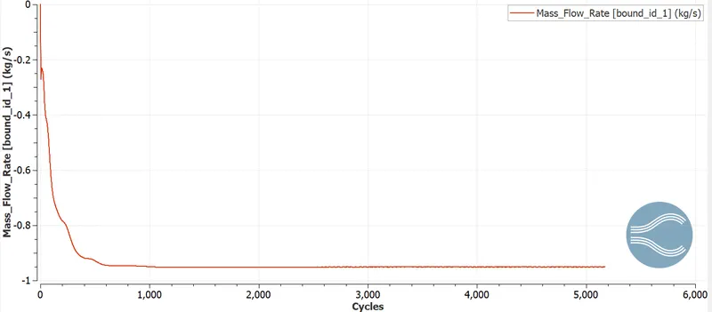
MASS FLOW RATE:

AT INLET:

 

AT OUTLET:

 

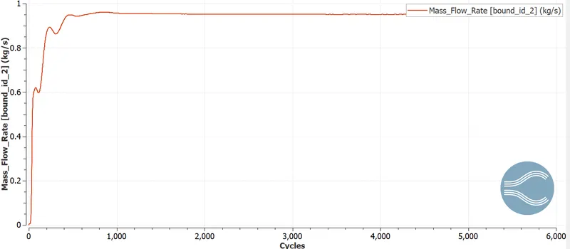
Mass flow rate at inlet and outlet are equal and the value is 0.95kg/s. the mass flow rate reaches the steady state after some cycles.

CASE 2:

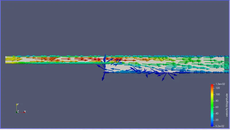
MESH: (1.5e-3 m)

 

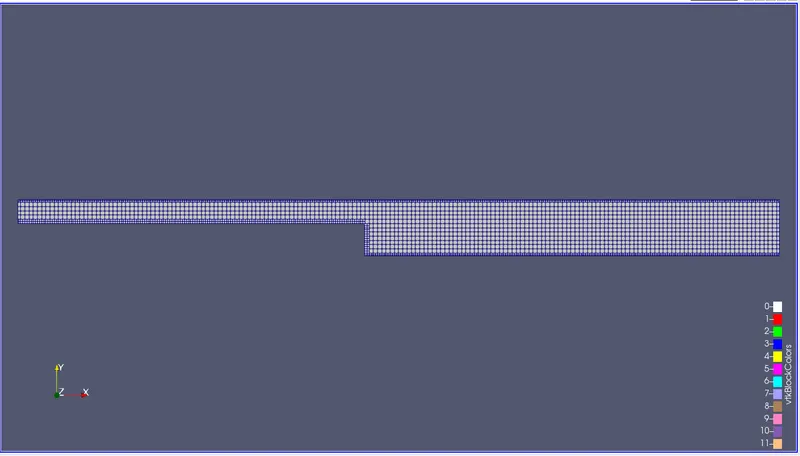
VELOCITY CONTOUR:

 

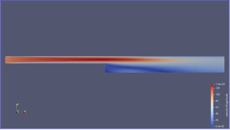
From the above plot we can say that velocity is high where the cross sectional area is less and velocity is less in the recirculation region.

PRESSURE CONTOUR:

 

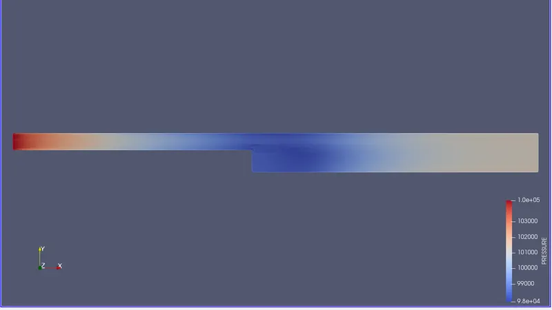
From the above plot, the pressure is less near the step or flow separation region. 

GLYPH:

VELOCITY PROFILE:

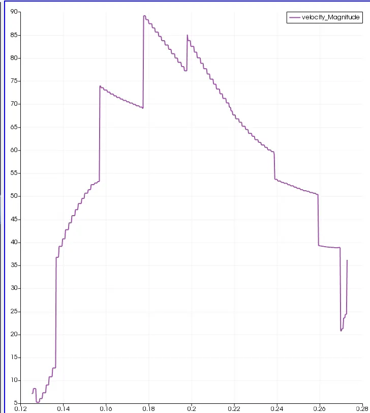
From this plot, the velocity increases near the step and then decreases.

PRESSURE PROFILE:

 

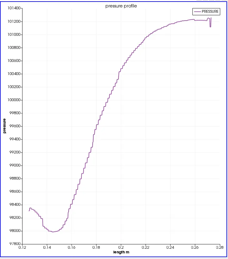
From this plot, we infer that pressure decreases near the step and then again increases.

CELL COUNT:

 

 

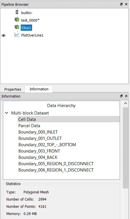
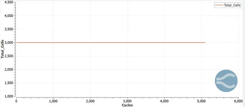
Number of cell count is 2994.

MASS FLOW RATE:

AT INLET:

 

AT OUTLET:

 

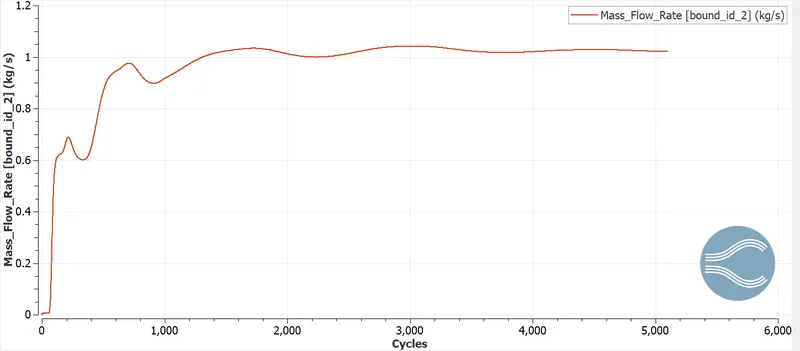
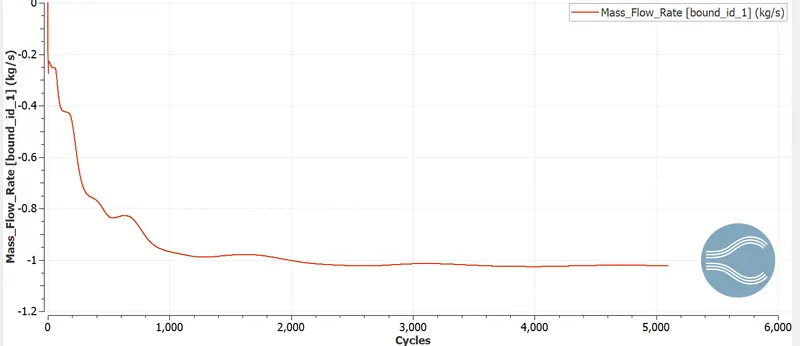
Mass flow rate at inlet and outlet are equal and the value is 1.05kg/s. the mass flow rate reaches the steady state after some cycles.

CASE 3:

MESH: (1e-3 m)

 

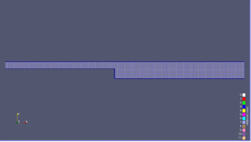
VELOCITY CONTOUR:

 

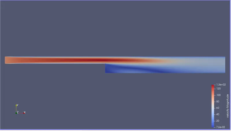
From the above plot we can say that velocity is high where the cross sectional area is less and velocity is less in the recirculation region.

PRESSURE CONTOUR:

 

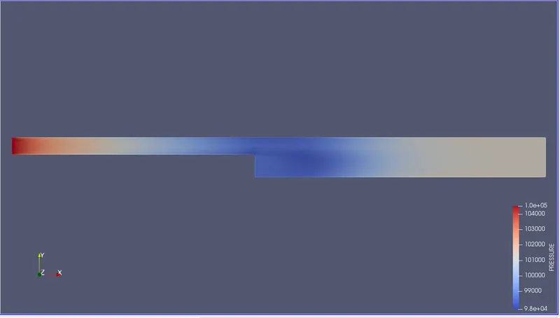
From the above plot, the pressure is less near the step or flow separation region. 

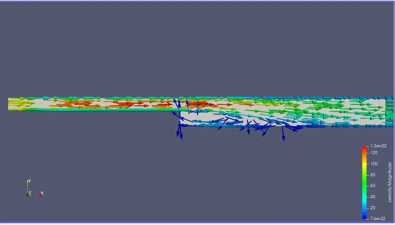
GLYPH:

VELOCITY PROFILE:

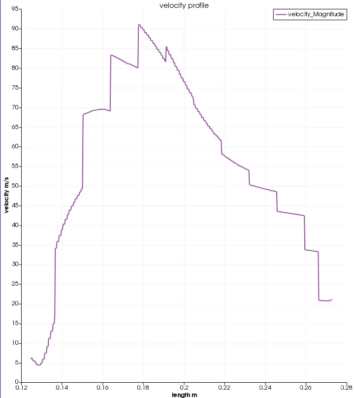
From this plot, the velocity increases near the step and then decreases.

PRESSURE PROFILE:

 

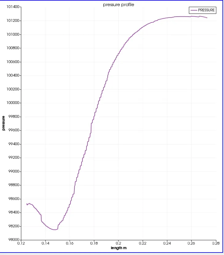
From this plot, we infer that pressure decreases near the step and then again increases.

CELL COUNT:

 

 

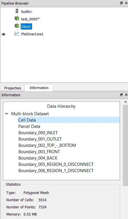
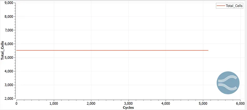
Number of cell count is 5516.

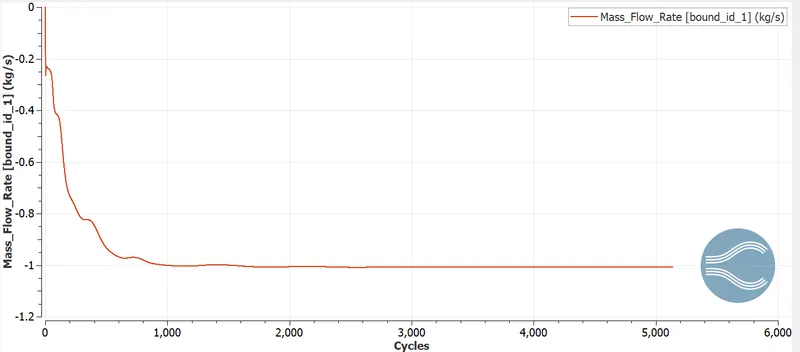
MASS FLOW RATE:

AT INLET:

 

AT OUTLET:

 

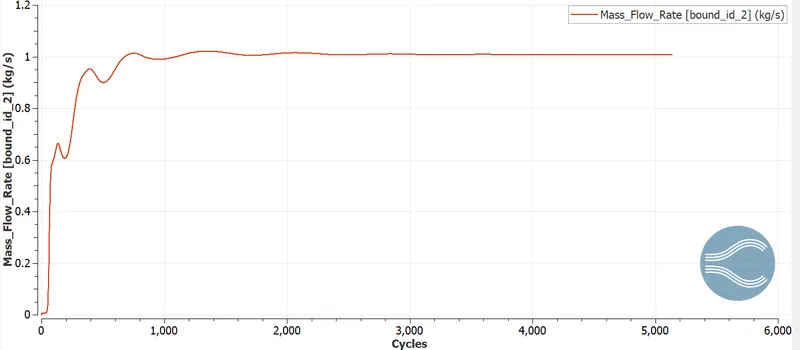
Mass flow rate at inlet and outlet are equal and the value is 1kg/s. the mass flow rate reaches the steady state after some cycles.

ANIMATION OF CONTOUR PLOTS:

 https://drive.google.com/file/d/1Seiew9U7UAtflaeQ88SN4tiXOVVi8WsV/view?usp=sharing

The animation shows how the velocity changes with respect to time.

CONCLUSION:

 From all the plots we can say that,

• As the mesh size decreases the results are becoming more accurate.
• As the mesh size decreases it increases the computational time.
• As the results are becoming more accurate the smoother plots are obtained.