Backward Facing Step Simulation with Three different mesh sizes in Converge CFD.

Aim: Flow over a backward-facing step.

Objectives:

1. The case should be run with 3 different mesh sizes.

• dx = 2e-4m, dy = 2e-4m, dz = 2e-4m
• dx = 1.5e-4m, dy = 1.5e-4m, dz = 1.5e-4m
• dx = 1.0e-4m, dy = 1.0e-4m, dz = 1.0e-4m

2. Post-processing of the flow parameters.

Introduction:

Backward-Facing Step (BFS) flow is one representative separation flow model, which is of significance in both theoretical and engineering development. Various applications for BFS flow can be found in our daily life, such as the airfoils at large attack angles, the spoiler flows, separation flow behind a vehicle, inlet tunnel flow of engine or inside a condenser/combustor, and also the flow around a boat or a building. It is a basic model that involves the most important features of a separated flow: free shear flow separation, vortex evolution, and re-attachment. As is well known that the flow separation near the BFS will possibly lead to additional flow resistance and noise, and under critical conditions even for stalling of an aircraft, the general understanding of the physics in BFS flow has become one hot topic in recent years. In addition, for some other applications such as mixing chambers or combustors, effective mixing is preferred and can be designed with detailed BFS geometric considerations, which also leads to the study of various mechanisms and controlled studies in this field. Backward-Facing Step (BFS) has also been partially discussed in general previous studies of flow separation dynamics. Flow separation is one classic topic in fluid dynamics, which has become one key topic in external flows and is closely related to the aerodynamic design of vehicles, mechanics, and other moving bodies. The free shear layer evolutions are the dominant factor in the separation process. According to Brown and Roshko, the shear layer indeed defines the coherent structures after a flow stability transition, vortex mixing, and pairing process.

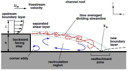
Bernal and Roshko then reported the 3-D structure and its extensions after separation, which governs the ensuing flow structure evolutions. Many studies on the detailed technical aspects of the separation process have been published in recent years. Among those, separation flow in external and internal flows shows different behaviors due to the confinement of walls and the specific design of model geometry. The researchers conducted a series of studies with compressible effects on natural convection with boundary flow separation/reversal under high Reynolds numbers and the microscale effects under confining walls that relate to the classic theory of Roshko and his colleagues. Such surface pressure changes and the separation bubble variations with Reynolds numbers and inflow conditions. Such compressible effects on heat transfer not only happen in the aerodynamic flow field but also happen in a wide variety of engineering conditions, such as chemical mixing, airfoil heating/cooling, and building. Such local boundary unstable flow under flow separation and reversal process with actuators/ heat control become very important when related to spacecraft re-entry process (with high Re and Ma number) where after-body steps are often seen. Such a series of studies lead to more general thinking about the general laws of flow separation in generalized models such as BFS, one most often seen in models for separation flow.

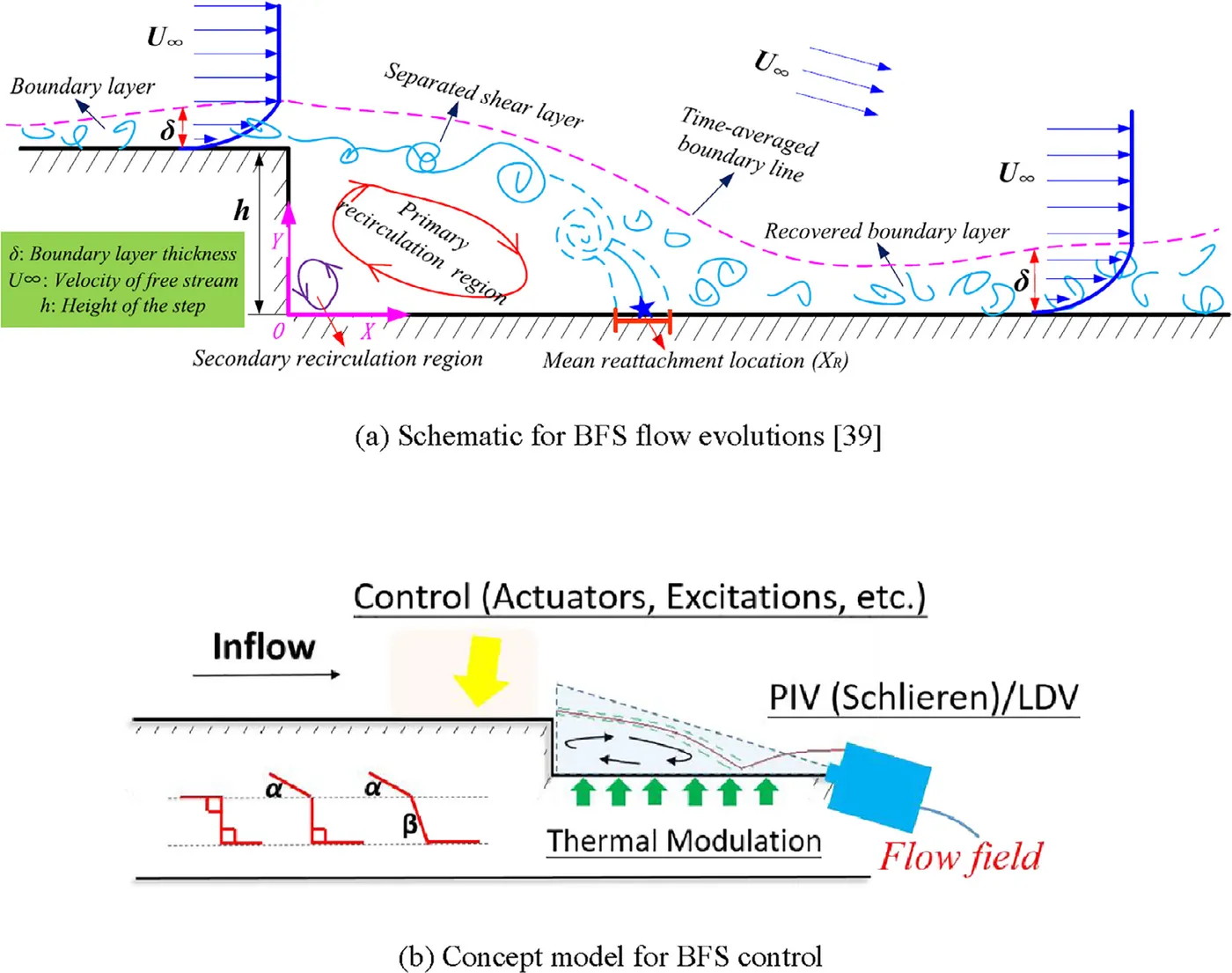
Importance of Backward Facing Step Problem

Separation and reattachment of turbulent flows occur in many practical engineering applications. It is seen both in internal flow systems such as diffusers, combustors, and channels with sudden expansions and in external flows like flow around airfoils and buildings. In these situations, the flow experiences an adverse pressure gradient, which causes the boundary layer to separate from the solid surface. The flow subsequently reattaches downstream forming a recirculation bubble. The presence of a separated flow, together with a reattaching flow, gives rise to increased unsteadiness, and pressure fluctuations which may lead to structure vibrations and noise.

-----------------------------------------------------------------------------------------------------------------------------

Case setup

The bfs. STL file is loaded into the Converge-CFD set-up.

The "Normal Toggle" is selected from the ribbon, upon selecting the normal toggle it was observed that the normal is pointing outside the volume, technically the normal should point inside the volume where the fluid is flowing. Therefore in the geometry dock, the "Transform" option is clicked. The "Normal" tab is selected from the geometry dock and one of the triangles containing the normal pointing outward is selected. The "Apply" option is selected for removing the normals.

The diagnosis dock is selected from the "View" option and the "Find" option is selected. It is found that there is no problem observed in the geometry ("Intersections(0)","Nonmanifold Problems(0)","Open Edges(0)", "Overlapping Tris(0)","Normal Orientation(0)","Isolated tris (0)".

The "Case Setup Dock" is selected from the "View" and "Begin Case Setup" is executed.

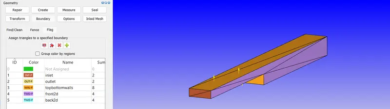
Fig1: Backward Facing Step Geometry

------------------------------------------------------------------------------------------------------------------------

Boundary setting:

• We have to set Inlet, Outlet, Top and Bottom walls, Front & Backface boundaries for the above-created geometry.
• By default In CONVERGE, all the surfaces are made up of triangles we have to select respective triangle faces for the boundary.

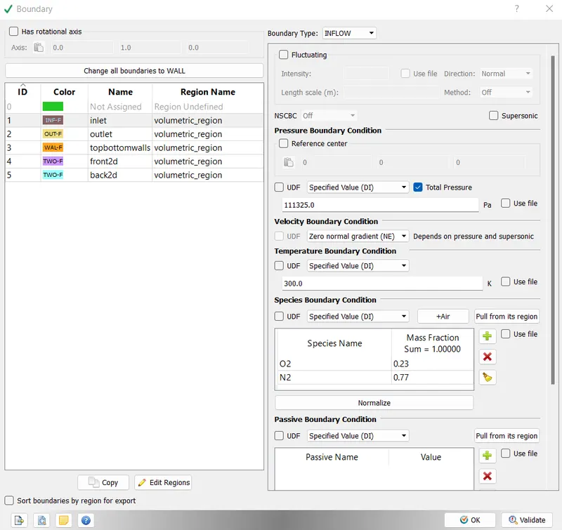
INLET

1. Inflow Boundary
2. Pressure = 110325 Pa
3. Mixture - Air

------------------------------------------------------------------------------------------------------------------------------

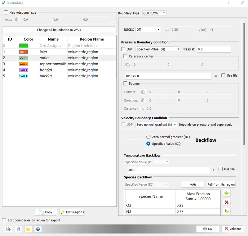
OUTLET

1. Outflow Boundary
2. Pressure = 101325 Pa
3. Mixture - air

------------------------------------------------------------------------------------------------------------------------------

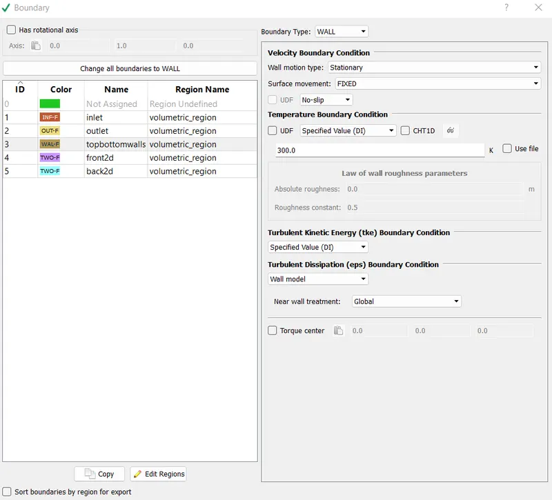
TOP AND BOTTOM WALLS

1. Wall Boundary
2. Temperature = 300 K
3. Velocity - Stationary
4. Temperature - Law of Wall
5. Turbulent Kinetic Energy - Zero normal gradient
6. Turbulent Dissipation - Wall model

---------------------------------------------------------------------------------------------------------------------------

Initial Condition

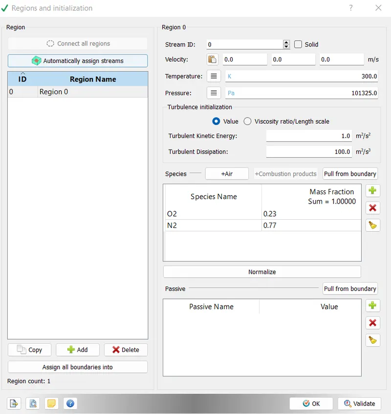
In the "Region and Initialization" the mass fraction of O2">O2 and N2">N2 were created and named as "Region 0" and the same is updated in the boundary condition region name. These are the initial condition and will be washed out after the solution has converged.

---------------------------------------------------------------------------------------------------------------------------

Monitor Variables

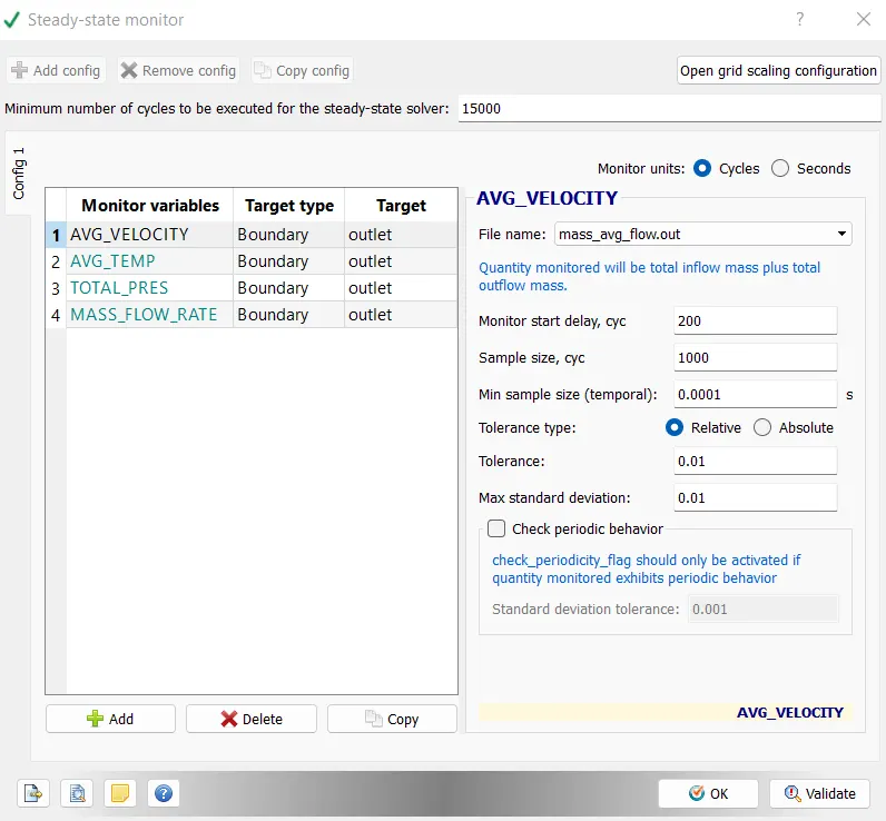
The monitor variables are added in the "Steady-state monitor". Avg Velocity, Mass flow rate has been added and the target area is selected as output. The minimum number of cycles to be executed for the steady-state solver is 15000 which signifies that the solver will run for a minimum of 15000 cycles if the solution reaches convergence value before 15000, then the simulation will stop at 15000, but if the solution reaches a convergence value after 15000 then it will terminate at that moment. The solver checks the difference in the value of two consecutive sample sizes (1000) and matches it with the tolerance value to stop the solution. The converge-CFD software saves a lot of time and computational energy by tracking the solution when it reaches a steady-state.

------------------------------------------------------------------------------------------------------------------------------

Simulation Time Parameters

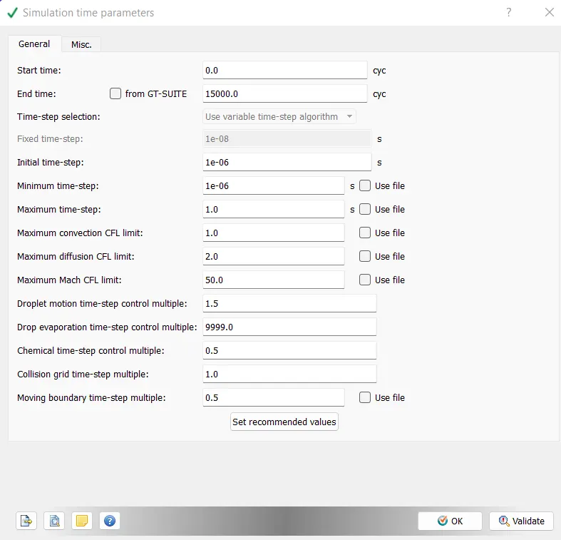
Under "Simulation time parameters" end time is chosen as 15000 cycles (steady-state). The initial and minimum time step is 1e-06 s. The maximum time step is 2s, and the maximum convection CFL limit is 1 and the rest are default values.

----------------------------------------------------------------------------------------------------------------------------

Turbulence model

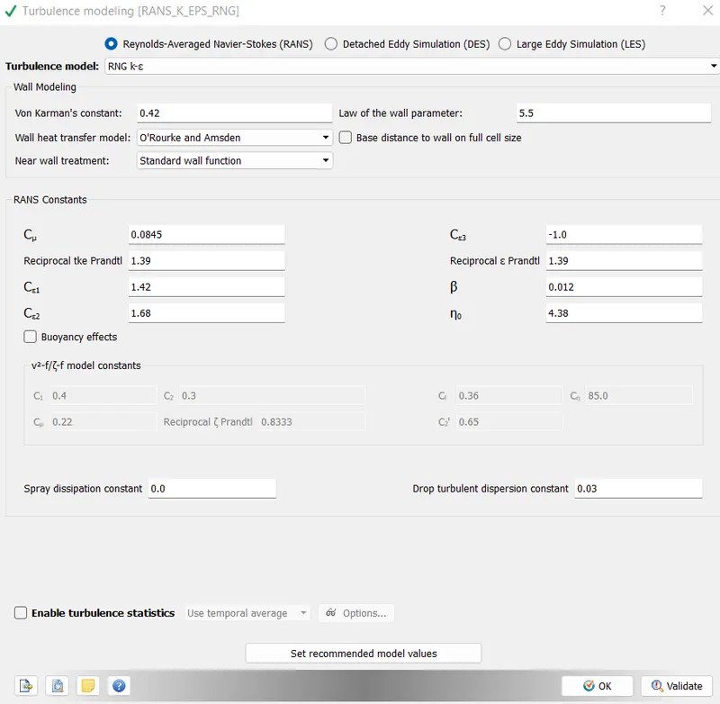
The Realisable k-ε">k−εk-ε model is selected from the case-setup tree for the above-said simulation. Since the size of the eddies is restricted near the wall and the maximum size of the eddies is formed away from the wall. It is well suitable for resolving flows in the logarithmic flow region where y+ ranges from 30 to 300, and for flows involving a high Reynolds number.

----------------------------------------------------------------------------------------------------------------------------

Grid Control:

Fixed Embedding

It is used to refine the grid at specific locations in the domain where a finer resolution is critical to the accuracy of the solution. In this case the regions of the interest are the inner walls of the channel.

For each fixed embedding, you must specify an embedding scale that indicates how CONVERGE will refine the grid in that location. The embed scale parameter, which must be a positive integer, scales the base grid sizes (dx base, dy_base, and dz_base)

Calculation of the fixed embedding is

26-3 dx embedded 2embedded scale

dx base

In our cases the dx values are 2e-3,1.5e-3,1e-3 and the embedded Scale values is 1.

The dx_embedded values are 0.001,0.0075,0.005

These are mesh values that refines the mesh at our desired location.

• In the Grid control enable the Fixed Embedding and Base grid
• Enter the base grid values and then go to the fixed Embedding add the
• Entity type=Boundary
• Boundary ID=Top and Bottom
• Mode =Permanent
• Scale=1
• Embedded layers=1

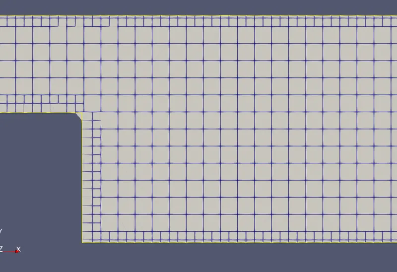
cell size=0.002m

...............................................................................................................................................................

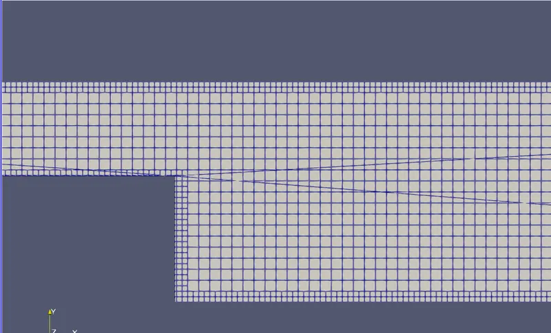
cell size=0.0015m

...............................................................................................................................................................

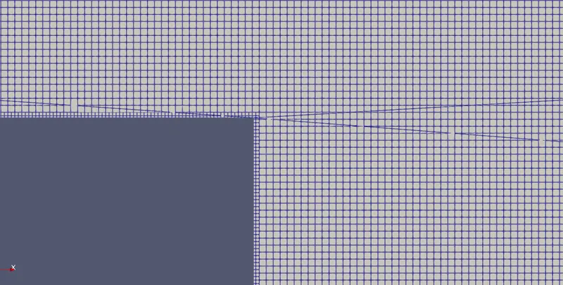
cell size=0.0001m

...........................................................................................................................................................

----------------------------------------------------------------------------------------------------------------------------

Solver Type

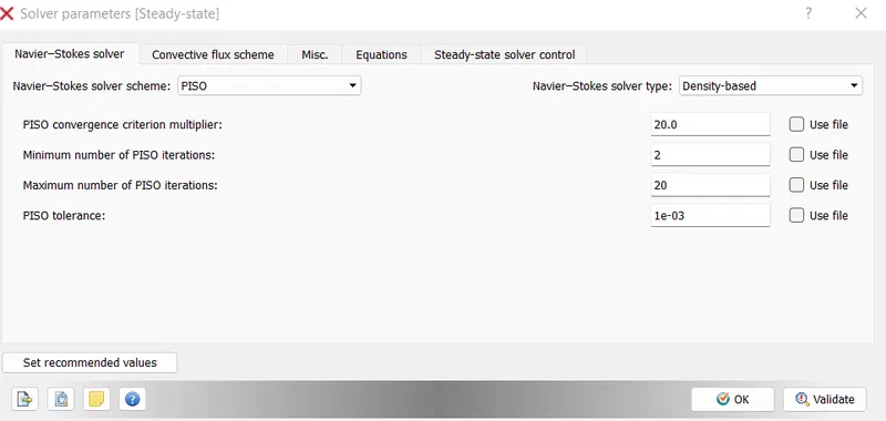
PISO involves one predictor step and two corrector steps and is designed to satisfy mass conservation using predictor-corrector steps.

The density-based solver solves the governing equations of continuity, momentum, and (where appropriate) energy and species transport simultaneously (i.e., coupled together).

-------------------------------------------------------------------------------------------------------------------------

Results

Mesh-1

Velocity

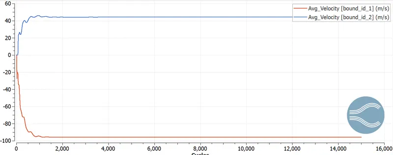
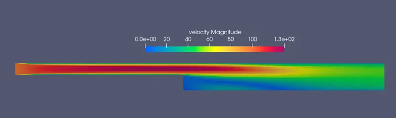
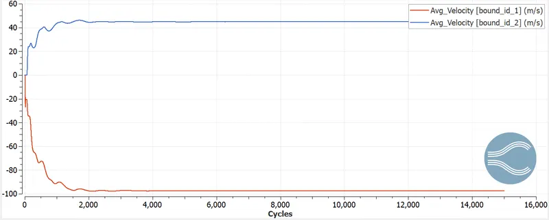The Velocity at the inlet is -95 m/sec and the velocity at outlet is 45 m/sec.The velocity is high in the inlet and low at the outlet because of the increased cross sectional area for the outlet when compared with the cross sectional area of the inlet.

Pressure

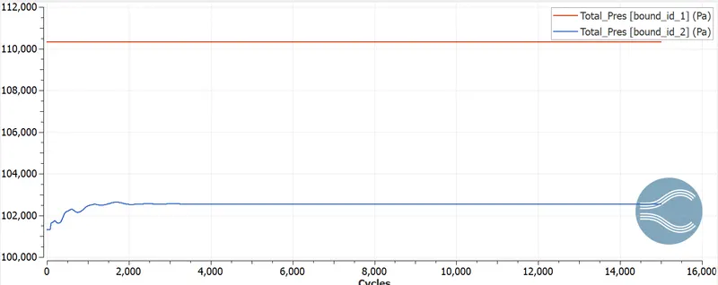
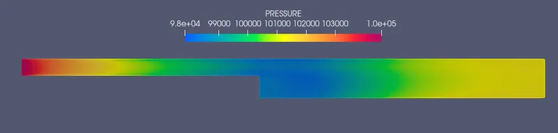
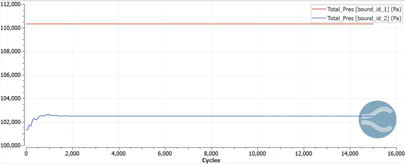
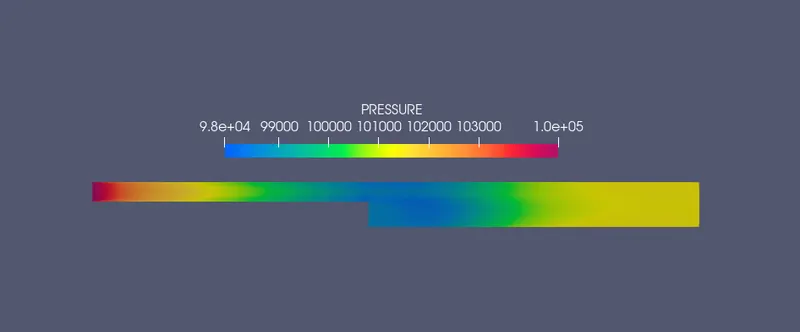
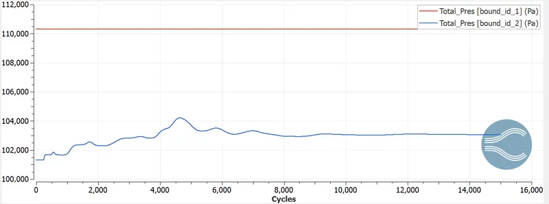
The pressure is constant at the inlet and the pressure at the outlet is gradually increased from the starting cycles and achieved the convergence after the 2000 cycles and reamins the same value throughout the simulation.

Mass flow rate

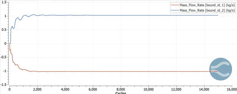
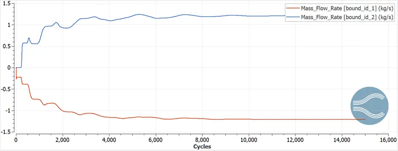
As the air enters the domain there is mass flow rate of 1.0 kg/s. When the air enters there is a negative sign, when the flow of direction is opposite to the normal. The opposite signs tends to cancel each other to say that the mass has been conserved.

Total cells

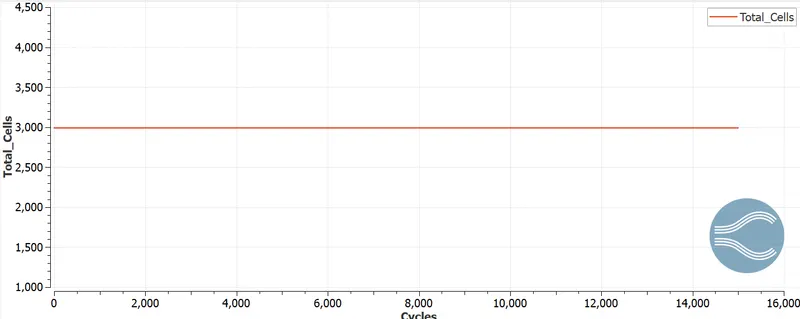
The total number of cells is around 3000 cells.The number of cells are low and the outputs of all graphs and plots are not smooth.

Mesh-1

Contour plots

Velocity

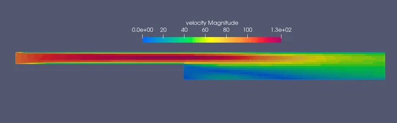
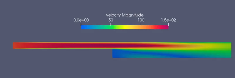
The velocity contours represents the flow in the backwardstep.The velocity is higher at the inlet with a 130 m/sec and at the outlet the velocity is gradually decline with a approximately of 55 m/sec due to the increased in the geometry and at the step the velocity is very low due to the divergent nozzle and the flow is turbulent so the pressure droping takes places so that the velocity starts decreasing from this point only.

Velocity Contour with Vectors

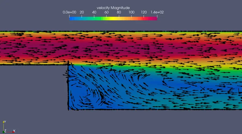
In the velocity countours with the vectors, the velocity after the step is recirculating because of the separation in the flow and form the boundary layer with the shear zone and at distance forming a vortex which is the region for recirculating the flow.

Pressure

Animation file

Velocity

Pressure

-----------------------------------------------------------------------------------------------------------------------

Mesh-2

Velocity

Pressure

Mass flow rate

Total cells

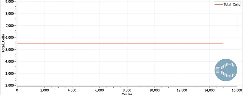
The total number of cells is around 5550 cells.The number of cells are high and the outputs of all graphs and plots are smooth.

Mesh-2

Contour plots

Velocity

Pressure

Animation file

Velocity

Pressure

------------------------------------------------------------------------------------------------------------------------------

Mesh-

Velocity

Pressure

Mass flow rate

Total cells

The total number of cells is around 5550 cells.The number of cells are high and the outputs of all graphs and plots are smooth.

Mesh-2

Contour plots

Velocity

Pressure

Animation file

Velocity

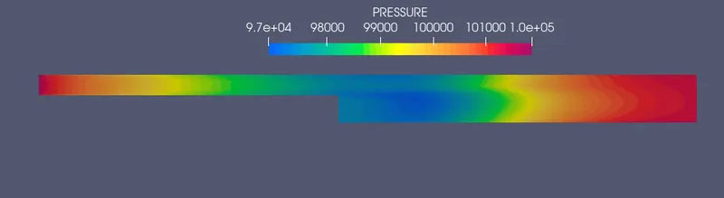
Air enters the inlet of backward-facing, due to the sudden changes in the geometry section at 0.1231m from the inlet, the air gets separated from the boundary leading to the deacceleration of the flow and reduction in the static pressure in that region, and beyond that, as seen in the above graphics file there are recirculation zones being formed and reattachment to the boundary layer occurs.

Conclusion

• The steady-state simulation of the backward-facing step was carried successfully using the "Converge-CFD" and "Cygwin" command prompt terminal.
• As air enters the inlet of the backwards-facing step experiences turbulent flow, the turbulent flow is characterised by choosing the proper turbulence model to visualise the flow.
• The Realisable k-ε model was chosen from the case setup tree and the default values were set accordingly.
• The turbulent flow initializes the formation of eddies near the wall and away from it. The size of the eddies are restricted near the wall and as we move away from the wall the size gets bigger.
• The flow gets separated from the boundary layer after the step due to a change in the geometry and after the step, there are a recirculation zone and reattachment zones leading to the deacceleration of the fluid and thus reduction in the static pressure.
• The total pressure loss is subdivided into irreversible pressure drops related to friction in the channels before and after the step, the reversible pressure rise at the expansion and an irreversible pressure drop occurring due to additional losses at the step.
• The turbulent structures in the shear layer catches the irrotational fluid from the non turbulent flow and this causes from the low velocity recirculation in the region.