Week 3 - External flow simulation over an Ahmed body.
Week 3 - External flow simulation over an Ahmed body.
Aim- To simulate the flow over the Ahmed body and analyze the factors affecting the flow.
Objective
Q1. Describe Ahmed's body and its importance.
Q2. Explain the reason for the negative pressure in the wake region.
Q3. Explain the significance of the point of separation.
Expected Results:
1. Velocity and pressure contours.
2. The drag coefficient plot for a refined case. ( For a velocity of 25m/sec, the drag coefficient should be around 0.33).
3. The vector plot clearly showing the wake region.
4. Perform the grid independency test and provide the values of drag and lift with each case.
Ahmed's body and its importance.
The Ahmed body was described originally by S. R. Ahmed in 1984, a real-life
automobile is a very complex shape to model or to study experimentally. Therefore study the vehicle-like shape was employed by Ahmed, known as the Ahmed body. Following is the Ahmed body with actual dimensions in mm included. Two different rear body slant angles (25° and 35°) were considered, which happen to bracket the critical angle of 30° at which separated flow occurs within the wake of the slant.
To study the actual car in wind tunnel test is complex due to its body design and employment of measuring accessories in a wind tunnel, hence to study the drag force and respective coefficient, most of researcher has created the dimension of car which can be studied as the replacement of actual one which called Ahmed body. In most of the simulation, the slant angle is changed to study the flow separation over the body.
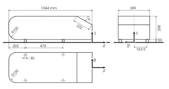
The Ahmed body was mounted in the test section of the LSTM wind tunnel and detailed measurements of velocity profiles were made around this body. The present studies were conducted in an open test section (i.e., floor, but no sides or ceiling) with a blockage ratio of 4%. The wind tunnel can generate flow velocities from 3 to 55 m/s with average turbulence intensities of less than 0.25%. To ensure the constancy of the test section bulk velocity and air temperature, a computer-based feedback control system was utilized.
Turbulence is one of the phenomena which need to be studied for the development of the car body and other features of car utility. The wake region behind the vehicle is very important to determine the slope behind the car. Ahmed body is a structure is mostly used to study the turbulence created by flowing air
Three main features are seen in the wake:
1. Recirculation region that is formed as the flow separates at the top of the vertical back surface of the model
2. Recirculation region that is formed due to the separation at the base of the model.
3. Pillar vortices that form as the vorticity in the side boundary layers roll up over the slant edges.
The wake was shown to be highly dependent on slant angle. For slant angles less than 12°, the flow remains attached over the slant. The flow is essentially two-dimensional and has low drag. Between 12° and 30°, the flow becomes much more three-dimensional as the c-pillar vortices form. These reach maximum strength at 30°. The drag increases significantly as the low-pressure cores act on the rear surfaces. Past 30° the flow separates off the slant. This results in a sudden decrease in drag and weaker c-pillar vortices.
SETUP
1. Geometry
- Load the CAD model in SpaceClaim & change units from mm to m.
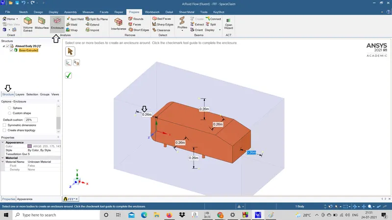
- Create a virtual wind tunnel using enclosure turn off the symmetry option from enclosure and create by a green check
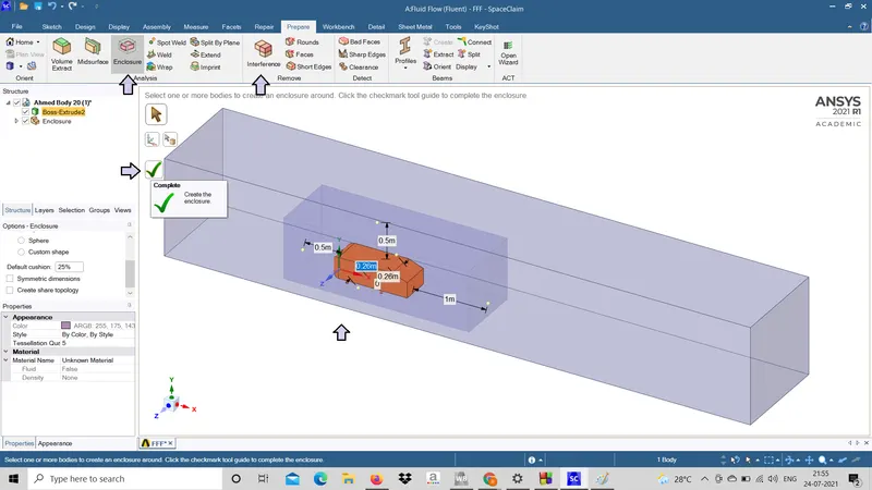
- After 1st enclosure create another enclosure using same procedure, as the dimension of larger enclosure are 5m at right (from face from car body) 2m at left, 0.05 width, 0 and 1m at bottom and top respectively.
- As the diameter of smaller enclosure is 1m at right (from face from car body) 0.05m at left, 0.26m width, 0 and 0.05m at bottom and top respectively.
- As we have created te smaller enclosure inside the large enclosure it overlaps the object hence results in mesh overlapping.
- To avoid use interference SpaceClaim detects any interference automatically, click green check to create the function
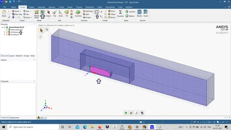
- To confirm create a plane select a plane along the length and create a sectional view.
- As the geometry is symmetry along its axis we can split the object this will result in creating fine mesh and converge the results faster; to split the object use split option given in SpaceClaim as shown below
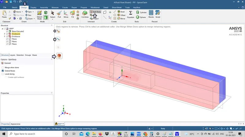
- Select split body -> select enclosure -> select plane along the x-axis -> select the side of object to be cut.
- An object will be created with a split.
2. MESHING
Y+
- Y+ is a non-dimensional distance.
- It is often used to describe how coarse or fine a mesh is for a particular flow pattern.
- It is important in turbulence modeling to determine the proper size of the cells near domain walls.
- The turbulence model wall laws have restrictions on the y+ value at the wall.
- For instance, the standard K-epsilon model requires a wall y+ value between approximately 30 to 300.
- And for K-omega model requires a wall y+ value between approximatly 0 to 5.
- A faster flow near the wall will produce higher values of y+, so the grid size near the wall must be reduced.
- We will be using K-epsilon model therefore value of Y+ be assuming as 75.
Calculations
- Calculating Re
we know that,
`U=25`
`L=1.044`
`mu=0.000017894`
`rho = 1.225`
`Re = (rho*U*L)/mu`
`therefore Re= 1786772.102`
- calculating cf
`Cf=0.026/(Re^(1/7))`
`therefore Cf=0.003325`
- calculating shear stress near wall
`tau_w=(Cf*rho*u^2)/2`
`therefore tau_w=1.2729`
- Friction velocity
`U_f=(tau_w/(rho))^0.5`
`therefore U_f=1.019`
- calculating first layer thickness For Y+ 75
`Delta Y=(y+ *0.000017894)/(1.225*1.019)`
`therefore DeltaY=0.001075`
- Thickness for 7 layers.
- `T_l=DeltaY*Gr^(n-1)`
| Sr. | n | thickness in mm |
| T1 | 7 | 3.2 |
| T2 | 6 | 2.6 |
| T3 | 5 | 2.2 |
| T4 | 4 | 1.8 |
| T5 | 3 | 1.5 |
| T6 | 2 | 1.2 |
| T7 | 1 | 1.0 |
| TOTAL THICKNESS | 13.5 ie. 14mm |
The total thickness of the Inflation layer for 7 layers is 14mm.
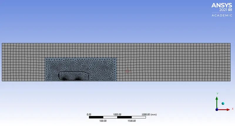
- After calculating the total thickness Open mesh and add multizone and create a method to the external enclosure
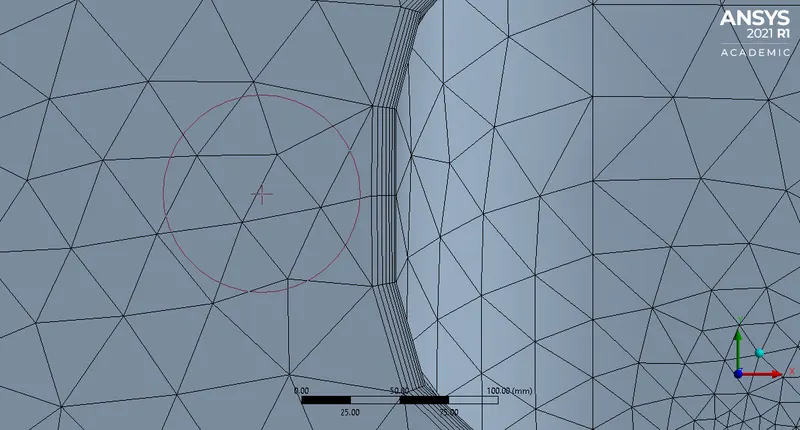
- Creat a Multizone method and change values of element size and maximum size according to cases as follows
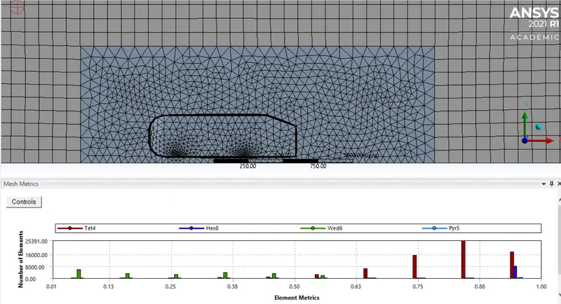
- After creating an Hexa mesh in external enclosure Create a mesh in the inner zine using body size and create mesh.
- as there is circular structure we have to body size the circular by selecting the inner surface area and apply and give values so that the mesh becomes sharper
- Now the mesh in external zone internal zone has been created but the car wall needs to be refined so we have to enter inflation layer
- let the layer be 7 and total thickness be 14mm as Calculated above.
- After creating method, sizing & inflation hit update mesh and mesh will be created.
- Let us consider 3 cases.
-
Cases Element size
(external encloser)
Body size
(internal encloser)
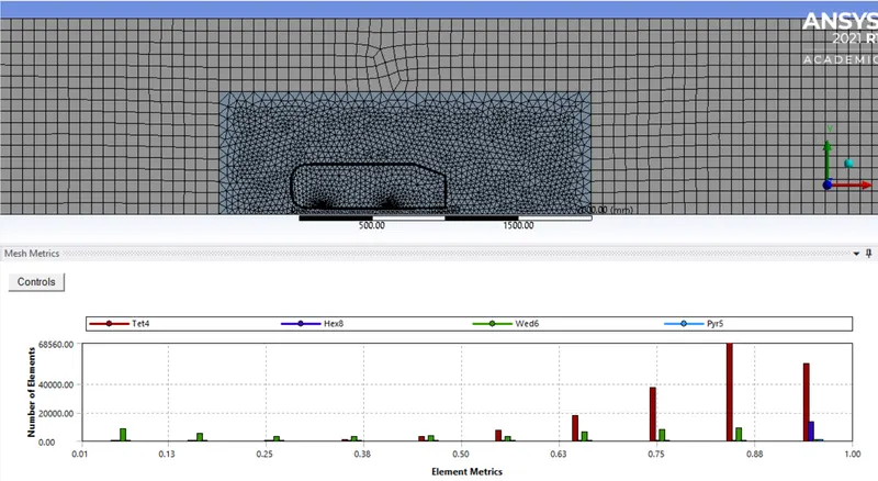
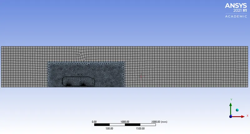
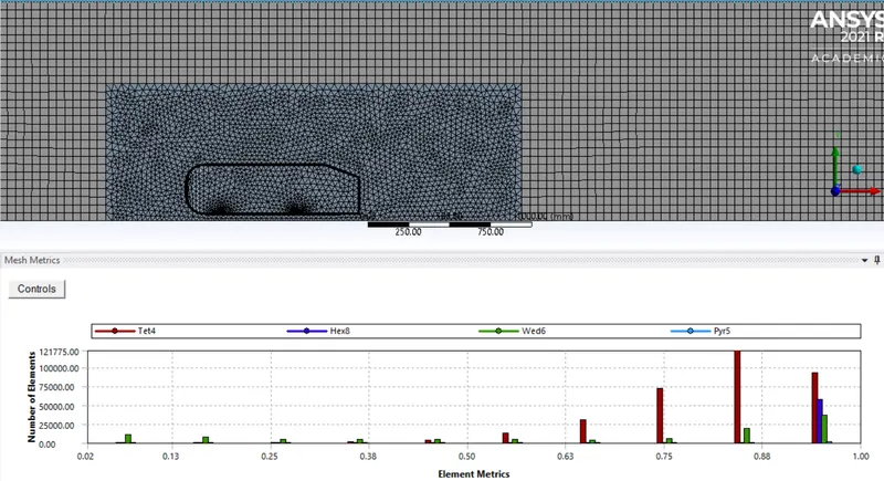
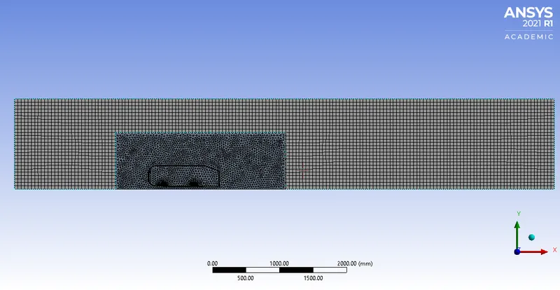
Face size Nodes Elements Thickness of layer Case 1 100 mm 50 mm 5mm 32653 95369 14mm Case 2 80 mm 35 mm 2.5mm 75144 249344 14mm Case 3 50 mm 30 mm 1.5mm 174001 486127 14mm
- Case 1
external enclose= 100 mm
internal encloser= 50 mm
Face size= 5mm
|
|
|
||||
 |
|
||||
 |
|
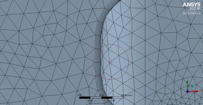
- Case 2
external enclose= 80 mm
internal encloser= 35 mm
Face size= 2.5 mm
|
|
|
||||
 |
|
||||
 |
|
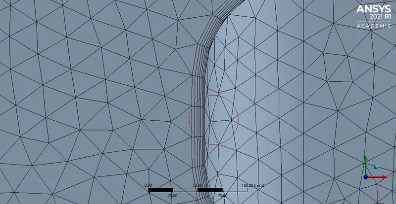
- Case 3
external enclose= 50 mm
internal encloser= 30 mm
Face size= 1.5 mm
|
|
|
||||
 |
|
||||
 |
|
- SETUP
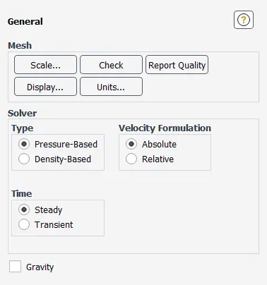
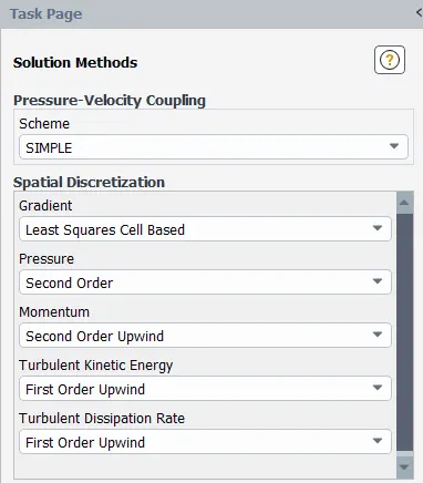
Using pressure based solver we have to perform all three cases.
General setting; After mesh -> update mesh and open fluent with double precision.
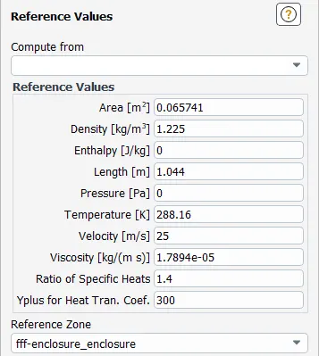
check the mesh and proceed for further set up as follows.
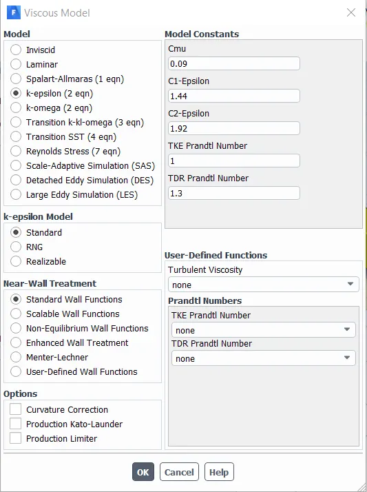
PHYSICS
|
 |
|
 |
|
 |
|
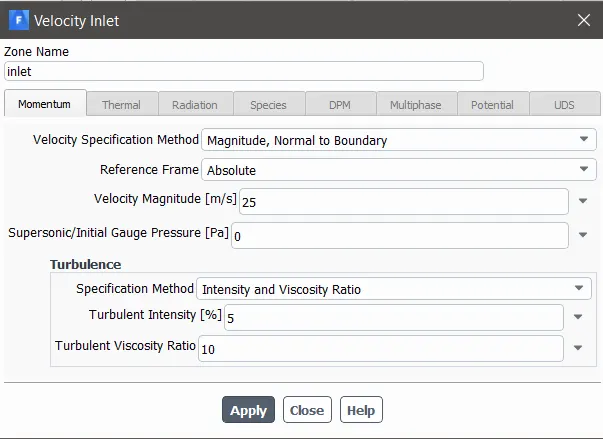 |
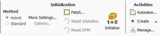
Before going to the solution, create an plane at z axis and contours, so hit initialize
Result
|
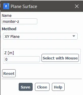 |
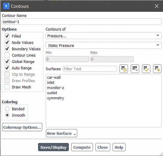
(creating contour for pressure and velocity in Z plane surface) |
 |
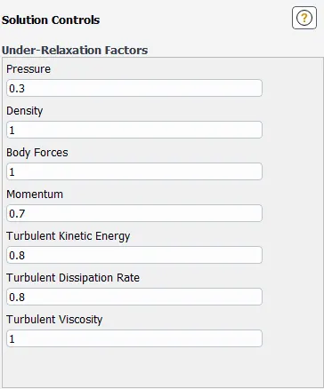
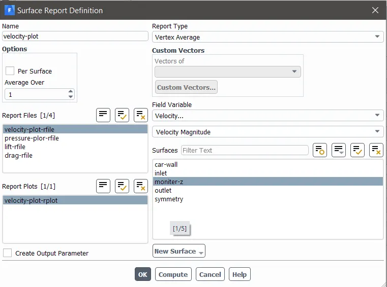
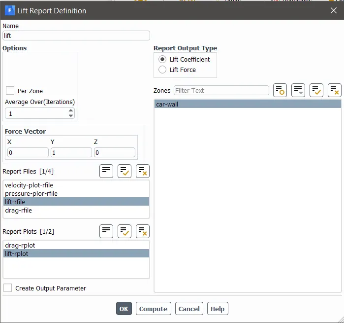
Now, setting up solution
SOLUTION
|
 |
|
 |
|
 |
|
 |
|
 |
|
 |
|
 |
RESULTS
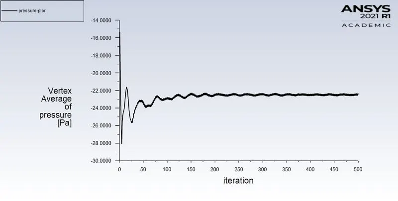
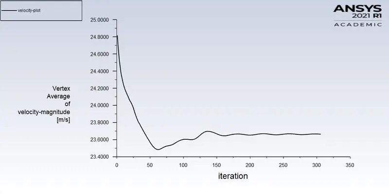
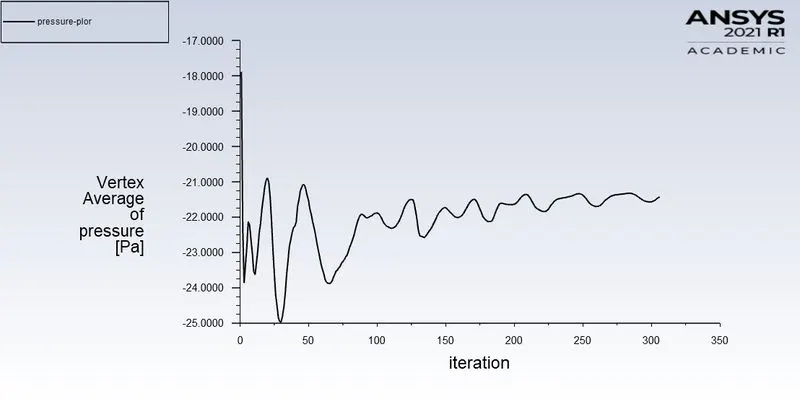
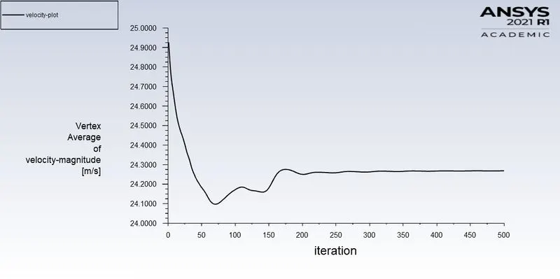
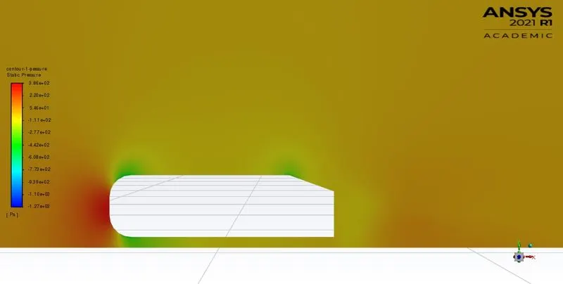
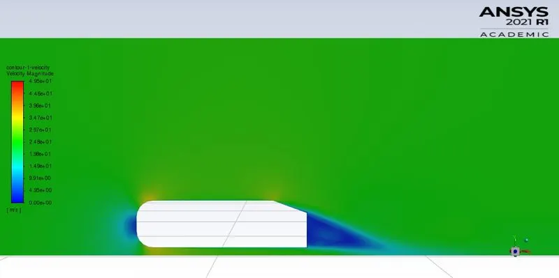
FOR PRESSURE AND VELOCITY
|
Case 1 |
|
 |
 |
| Case 2 | |
 |
 |
| Case 3 | |
 |
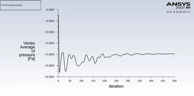 |
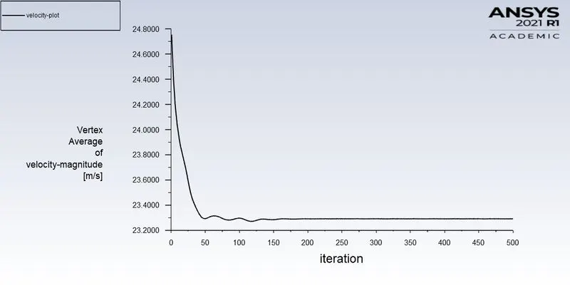
- As we see from above plot the velocity as well as pressure is high at the start and there is a sudden fall in pressure as well velocity
- But velocity gets stable but pressure gets changing this is due to the wake region where pressure drop can be seen.
PRESSURE AND VELOCITY CONTOUR
|
Case 1 |
|
 |
 |
| Case 2 | |
 |
 |
| Case 3 | |
 |
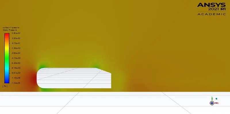 |
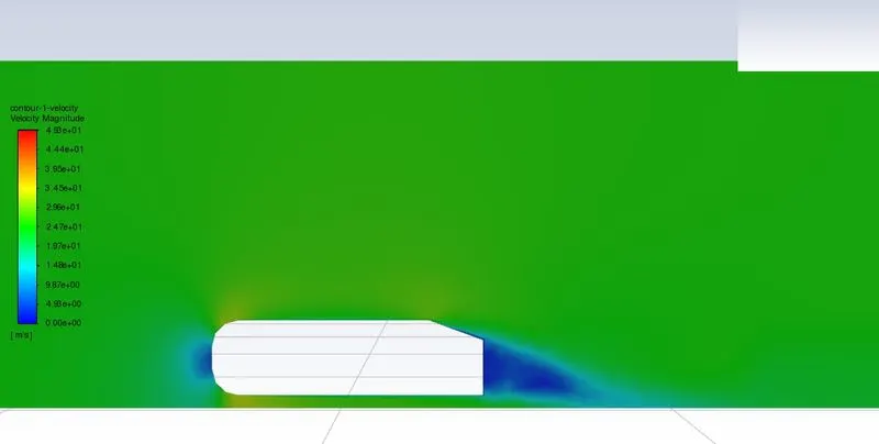
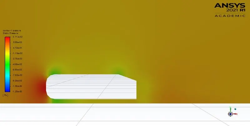
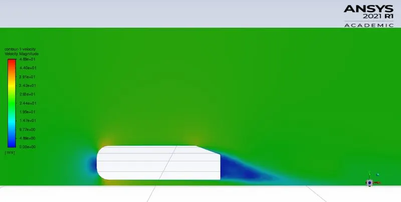
contours for 3 cases look similar but as we see at the wake region we see the case 3 velocity contour shows the curve to know more we have to look more in post and see what exactly happening in that region. Whereas pressure contours look similar with a minor change in values.
RESIDUALS
|
|
|
|
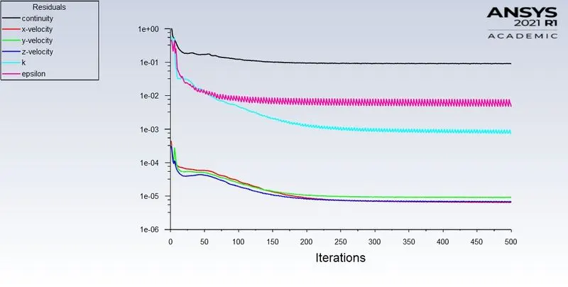
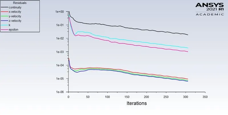
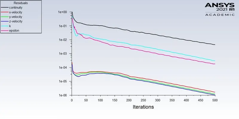
In the residual plot, for case 1, we see a lot of fluctuation in results. In contrast, other two study shows a small fluctuation.
- LIFT & DRAG
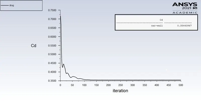
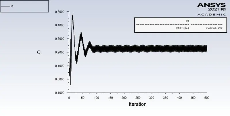
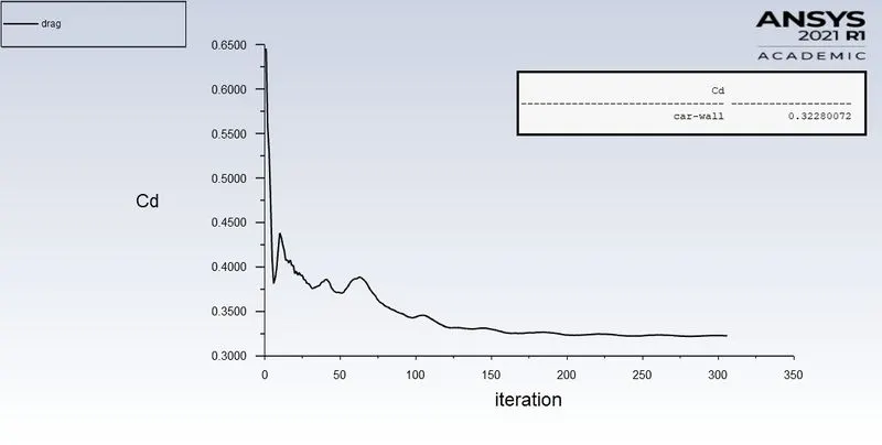
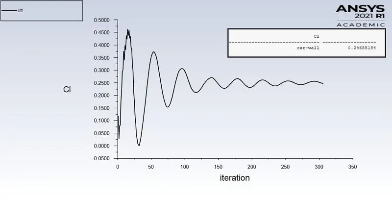
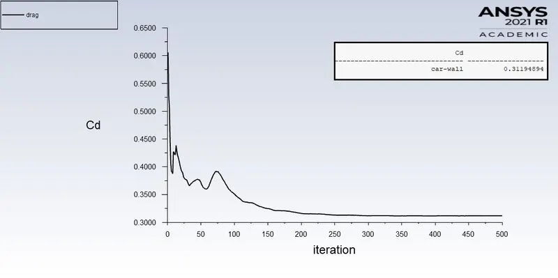
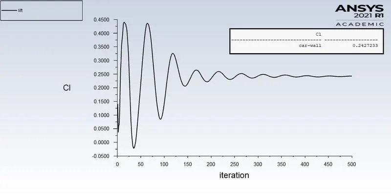
The drag coefficient quantifies the resistance of an object in a fluid environment. It is not an absolute constant for a body's shape because it varies with the speed and condition of flow, abject shape and size, and the density and viscosity of the fluid. The lower the drag coefficient of an object, the less aerodynamic or hydrodynamic drag occurs. In terms of a car, the lower the drag coefficient, the more efficient the car is. As well as affecting the top speed of a vehicle, the drag coefficient also affects the handling. Cars with a low drag coefficient are sought after, but decrease the drag drastically can reduce the down-force and lead to a loss in road traction and a higher chance of car accidents.
|
Case 1 |
|
 |
 |
| Case 2 | |
 |
 |
| Case 3 | |
 |
 |
- The above Drag coefficient at velocity of 25 m/s we can see that the as mesh gets finer the plot to gets precise
- As the mesh gets finer drag and lift coefficients gets more precise as we see in case 1 and 2 the lift coefficient have fluctuations.
- Case 1 has a lot of fluctuations as in case 2 we can small fluctuation but after it got smother. in case lift 3 is smothe.
MESH INDEPENDANCY TEST
In this project we considered three cases with different numbers of elements to verify that converge results are not varying because of grid size.
-
Cases external encloser-internal enclosure
No. of Elements Drag Coefficient ift Coefficient Case 1 100 mm - 50 mm 95369 0.354 0.202 Case 2 80 mm - 35 mm 249344 0.323 0.247 Case 3 50 mm - 30 mm 486127 0.312 0.243
The above table we can see the drag coefficient and lift coefficient we can see that both values reduces as the mesh elements increases, but increases computational time.
WALE REGION
The wake region is a distributed flow region or usually turbulent flow around a solid body moving through a fluid. This phenomenon is mostly caused due to the boundary layer separation which creates a high turbulent flow zone. This separation is caused by the adverse pressure gradient (High-pressure drops) giving a net pressure force. The velocity and pressure in this region are low and increase the drag force on the body. Since the drag force also depends on the wake region, the Formulation of the wake region is one of the important characteristics to consider while designing an automobile.
The negative pressure in the Ahmed body is due to bluff bodies. The boundary separation and recirculating of the flow and also the effect of shear stress. To overcome the shear, stress pressure turns negative to balance the effect.
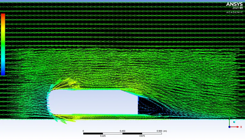
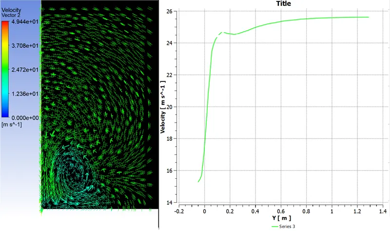
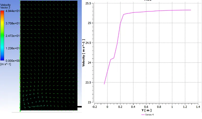
- As the mesh of case 3 has element size of 0.49Million cells let us take this case under consideration and check how flow behaves in wake region using vector and plotting velocities across the plan
 |
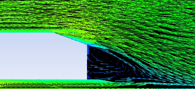 |
- The wake region increased the thrust force caused by the body depicted in the vector plot and the drag which extends behind the body. This makes the back-flow which travels from high to lower pressure region and the vortex is formed.
The point of separation
The point of separation is a point where the fluid flow no longer follows the contour of the body and gets detached from the surface of the body. When there is a fluid flow over a solid body there a retarding effect on the fluid flow that detaches from the surface giving rise to vortices and Eddie forces. Once the fluid is detached it exerts constant pressure on the surface instead of exerting a continually increasing pressure.
The boundary separation and recirculating of the flow and also the effect of shear stress. To overcome the shear, stress pressure turns negative to balance the effect.
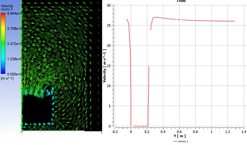
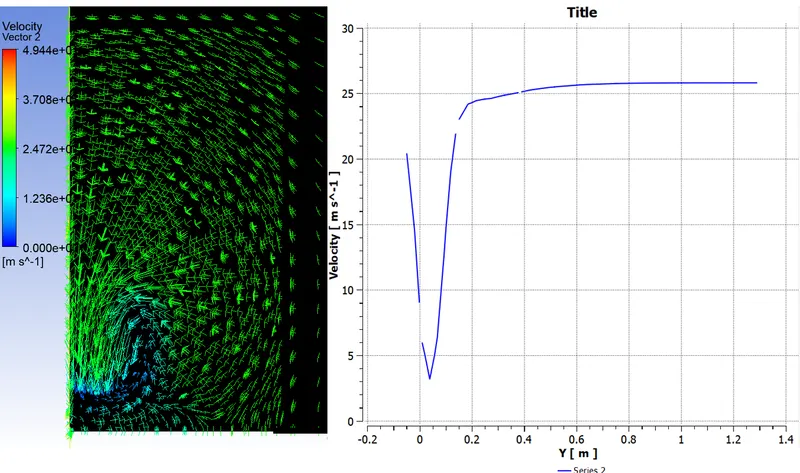
Velocity at various distance
|
 |
|
 |
|
 |
|
 |
CONCLUSION
- We can use a sectional part of the geometry if the geometry is symmetrical it helps in increasing mesh grid element cells also leads in reducing the computational time.
- We can verify the results got from the simulation to validate our simulation setup for actual geometries of Ahmed body.
- Using Y+ value to generating mesh improves the accuracy at the car-wall surface when the flow is turbulent, it also affects the accuracy of drag and lift coefficients.
- A grid independence test is important to validate the generated mesh of the final setup as it stablises the resuls.
- A hight turbulent zone is created at the wake zone & there is negative pressure created due to boundary layer separation.
- The boundary separation and recirculating of the flow and also the effect of shear stress. To overcome the shear, stress pressure turns negative to balance the effect.