Week 3 - External flow simulation over an Ahmed body.

Week 3

External flow simulation over an Ahmed body.

Objective:

In this test, We are going to talk about Ahmed's body and the significance of it.Explain why there is a negative pressure in the wake region, and provide a vector plot that shows the wake region in a way that is easily understood.Describe the significance of the point where the two paths diverge.In order to validate the drag coefficient, we will first simulate the velocity and pressure contours of the flow as it passes over Ahmed's body.In the conclusion, we will carry out the individual load test and report the values of drag and lift beside each scenario.

Introduction:

AHMED BODY

It is necessary to perfect the aerodynamics of the vehicle's exterior in order to produce highly efficient automobiles with low rates of fuel consumption, CO2 emissions, and noise while preserving a high level of driving stability. The importance of modelling the aerodynamics of a vehicle's exterior and calculating its aerodynamic characteristic numbers has been growing in tandem with the processing power available to do so. At the moment, effective management of resources is becoming increasingly important in every context. As a result, a sizeable portion of the time spent developing new automobiles is dedicated to the process of optimization. Virtual development is the only method, and the most effective one, for accomplishing this. In order to implement development processes such as these in the automotive industry, dependable simulation models that have been verified by experiments are required. Experiments that provide validation data use model bodies with variable parameters, like the back slant angle. For both numerical predictions and experimental studies, the wake flow behind a car is the most problematic flow region due to its large contribution to the vehicle's overall drag. The size of the separation zone and, as a result, the amount of drag force are both determined by the location of the point at which the flow separates. For the accuracy of drag predictions, it is abundantly clear that a simulation of the flow of the wake and of the separation process that is more precise is essential. However, a real-life automobile has a very complex shape that is difficult to model or investigate; experimentally, one such body is the Ahmed body. The Ahmed body is a bluff model body with a simple shape that has the fundamental aerodynamic properties of a vehicle. It has been used as a reference in a great number of investigations. The body of Ahmed is a three-dimensional model that is a representation of a typical model of passenger vehicle. This project's objective is to develop, improve, and validate the most recent generation of turbulence models for specific examples that are encountered in the field of vehicle aerodynamics. The availability of detailed experimental data is a prerequisite for the validation of turbulence models. In addition to that, this is utilised in the validation of CFD codes. In order to know whether or not your code is trustworthy, you must first compare its output to the data from the experiments performed on Ahmed's body. If it does, then you can put your faith in your code and use it to check whether or not other geometries are valid. This is an actual research model that was constructed in the real world; many people have conducted experimental analysis on it, and as a result, we have a significant amount of valuable data. Therefore, it can be of great assistance when validating CFD codes.

Boundary Layer Separations:

When a flow is confined by a wall, the pressure exerted on the fluid can change as a result of the curvature of the surface or an external force.When the freestream pressure rises in the direction of flow, this is called an adverse pressure gradient.When the pressure gradients go in the wrong direction, the flow slows down. When the velocity gradient at the wall gets close to zero, the flow will rise above the surface, sending the streamlines away from the wall. This process is called separation.As soon as a boundary layer separates, the corresponding equations can no longer be applied. However, we are able to estimate the location of the point of separation by observing the velocity gradient (or shear stress) at the wall of our solution and making a mental note of the location where it approaches zero.The pressure field in a fluid flow past an object is not uniform. When the pressure gradient is not zero, the velocity profile is affected.

In general, boundary layers separate when the speed of the boundary layer "struggling" against an unfavourable pressure gradient becomes close to zero, meaning that the pressure rises as the wall fades away, which pushes the fluid back.If the fluid's momentum isn't strong enough, the fluid will change direction and move away from the wall.he transition zone between the two flows is identified as the point when the shear force on the walls is equal to zero.At the point of separation, the boundary layer thickens dramatically, and the layer is pushed away from the wall by the reversal of flow near the surface.Laminar and turbulent flow regimes are distinguished by the presence of distinct vortical features in detached flow.

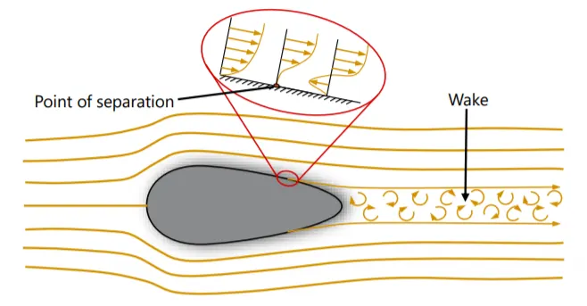
The significance of the point of separation:

When it comes to our situation, we are able to quickly understand that, at sharp bends and turns, the flow naturally divides. This is something that can be simply comprehended thanks to the concept of momentum conservation.This impact is exactly the same as flow in a problem with backward steps.As the boundary layer approaches the corner, it continues to move in the direction of the flow; without an external pressure gradient, it will be unable to maintain attachment and will instead break free.Because the flow is generally linear, a low-pressure area develops behind Ahmed's body.The area of low pressure then generates a recirculation zone by sucking in the straight-line flow.As a result, the Ahmed body's backside develops a sizable wake, and the recirculation zone becomes visible.The wake's emergence is graphically represented by the velocity profile.

Method of solving the problem:

Using a steady-state scenario, we will model the flow around Ahmed's body.

Then, in order to solve the problem, we will proceed as follows:

• Development of geometry
• Meshing
• Problem setup
• Solving
• After-effects processing

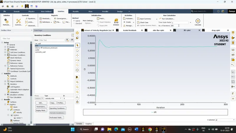
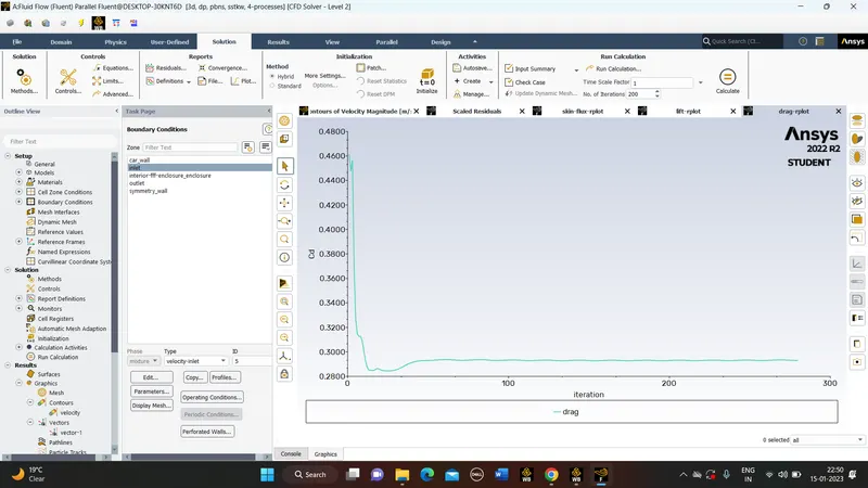
Then, while the model is being simulated, we plot the coefficient of drag and lift plot to demonstrate that the flow has converged and reached a steady state.

After that, we will do some post-processing on the results, during which we will also determine the drag coefficient and evaluate how it compares to the experimental value.

After that, as a concluding point, we will talk about how the Reynolds number influences the drag coefficient.

In the end, we will carry out the grid independence test and display the figures of drag and lift alongside each scenario.

When we simulate the flow using the Steady case, we see:

The fluent module is initially opened in the ANSYS work bench by using the drag-and-drop method.

Then, we carry out the procedure described in the previous paragraph.

CASE-1 :

Mesh size for enclosure 1 = 100mm & for enclosure 2 = 10mm ,Model =k-epsilon

1) The setup for geometry:

• The space Claim client needs to be opened in fluent module before the geometry can be imported
• 
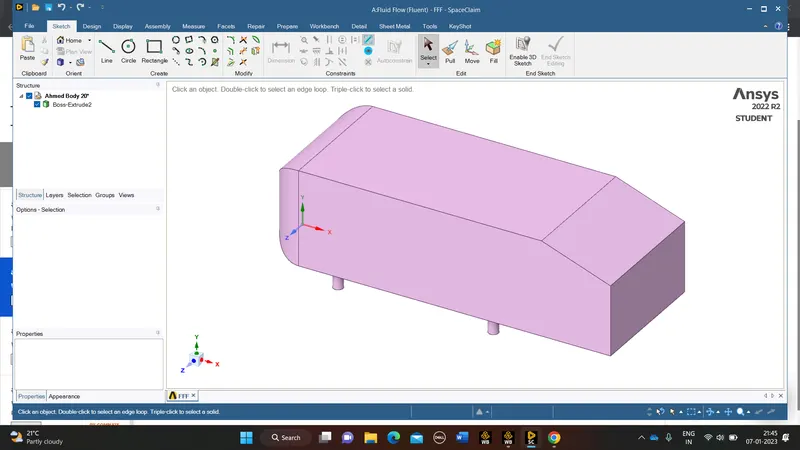
• Developing an enclosure across Ahmed body
• 

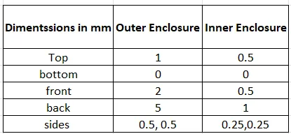
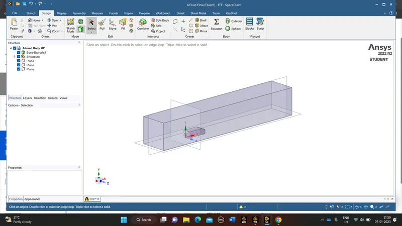
• To create an enclosure, we first click on Prepare, then select Enclosure, and then we de-select the Symmetric option in the Left Side Tree Bar. This allows us to control all the side dimensions and assign the data. At this point, you should click the green checkmark for implementing.
• Using interference Therefore, the two enclosures will work together to form a single boundary layer, allowing for smooth data transition analysis.

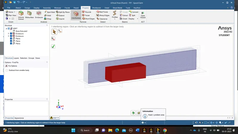
• We make use of the share topology so that all of the info can be shared among the various boundary layers.

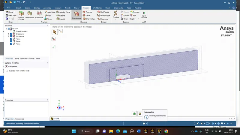
• To Split the body we need to create plane.

2) Meshing:

• In order to mesh our model, we first open the Mesh tool, which allows us to mesh it and then use it to solve our model.
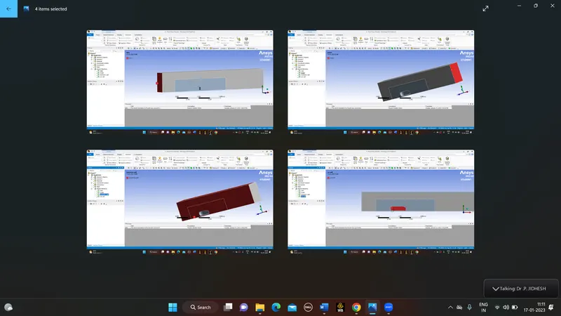
• We begin by selecting the entity using the entity selection through the use of faces in order to provide a name for our entity selection.
• procedure: using the edge selection tool, select the edge you want to name; then press the N key; finally, give the selection a name.
• In a manner analogous to this, we refer to our inlet walls, outlet walls, symmetry walls, bottom walls, and Ahmed bodies as our car walls.

• Then the following step is to mesh the materials.
• We begin by developing our base line mesh by selecting the mesh option located in the side window.
• Next, we will refine the mesh.
• Let us combine all of the geometry into one.
• As soon as the mesh is finished, we will need to determine what aspects need to be improved upon.
• Let us go through each step-in order.

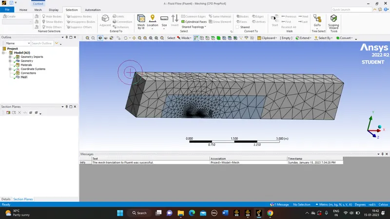
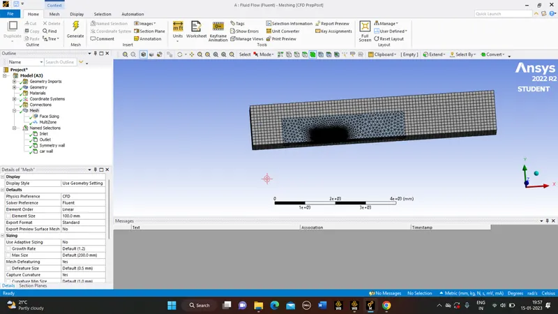
Sizing (Body sizing):

• By using sizing, we are making the mesh that is contained within the smaller enclosure even more fine.
• To accomplish this, right-click on mesh and then select sizing. Within the realm of geometry, we choose the inner box or enclosure and specify a size accordingly. After that, generate the mesh once more, and you will notice that the inner enclosure has been refined further.

Sizing(Edge Sizing):

• If you look closely, you'll notice that the cylinder pillars have been approximated using polygons. This is due to the fact that the element size is relatively large in that region.
• To resolve this issue, we used the single select tool to isolate the problematic faces, set the mesh size to 5 millimetres, and then generated the mesh. After doing so, you will notice that the affected faces are significantly improved and can now be interpreted as cylindrical pillars.

Inflation:

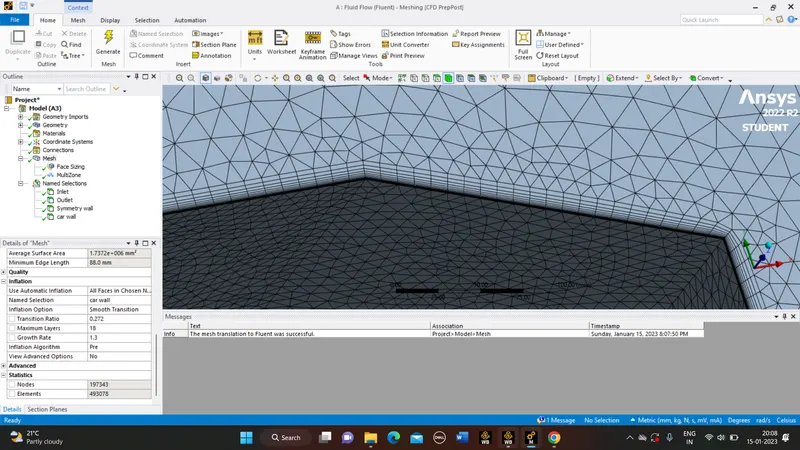
With the help of the inflation layer, we were able to create a mesh that was body-fitted. This indicates that it produces a layer of mesh that is identical to the geometry that surrounds the Ahmed body.

Because the flow around the Ahmed body is so significant, we need to focus on that region when creating inflation layers in order to ensure that we accurately capture that flow.

In order to accomplish this, we will need to right-click on mesh and then select sizing. When it comes to geometry, we go with a small enclosure, and when it comes to the boundary, we go with Ahmed's body boundary layer.

In addition, for the inflation option, the first layer thickness is what we use, and we determine it based on the y+ value and the turbulence model that we employ.

Because we are working with the k-omega model here, the value of y+ should fall somewhere between 0.1 and 5.

by using online y+ calculator we are using 0.4mm as a first layer thickness.

3) Problem Setup:

To begin the process of setting up our problem, we launch Fluent and configure the initial conditions, boundary conditions, material, and so on.

First things first, we run a quality check on the mesh by using the perform mesh check under domain command.

If there is no indication of an error in the console window, then we are free to move on.

The next step is to configure the physics, during which we make choices regarding the solver, viscous model, initial and boundary conditions, and so on.

In order to solve our model, we make use of a pressure-based solver that operates in a steady state.

Physics:

General:

Solver type : pressure based

time : steady state

velocity formulation : absolute

models:

viscous model: k-omega

Material: Air

Zones:

Cell zone: you will see our volume zone which is basically our internal volume basically mesh, and it is of type fluid.

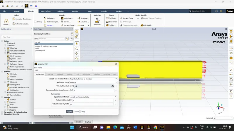
Boundary conditions: We will basically give our boundary conditions here such as inlet velocity and outlet conditions.

we give,

Inlet :

velocity : 25 m/sec

Outlet :

pressure outlet : gauge pressure = 0 pa

Car walls :

wall : No slip

Symmetry walls :

type : symmetry

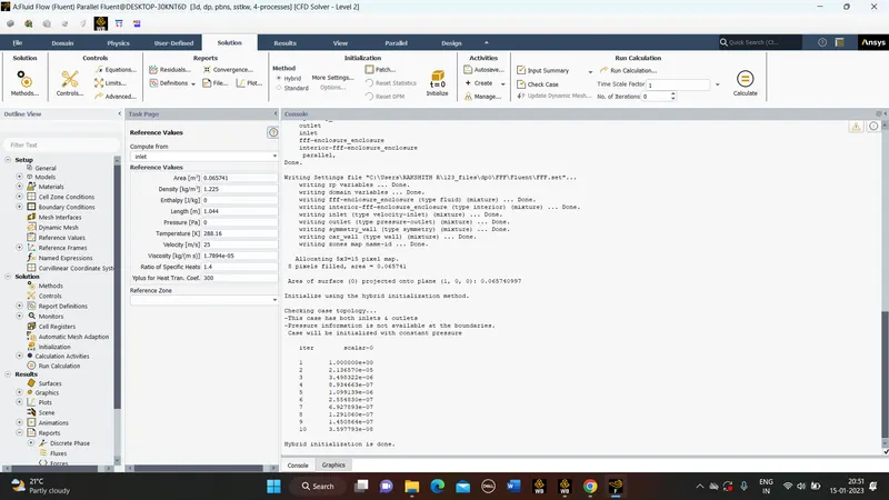
After these we need to create drag and lift plots and we perform an initialization, and then we solve for a total of 350 times as well.

4) Solving :

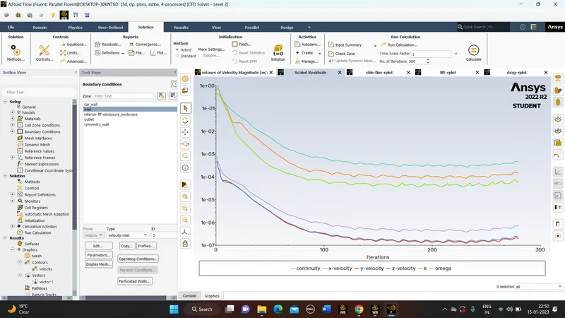
You should perform iterations in such a way that your solution converges.Carry on with the simulation until you have reached the steady state.The results are then subjected to post processing.

5) Post processing:

• Residuals
• 
• lift-rplot:
• 
• Drag-rplot:
• 
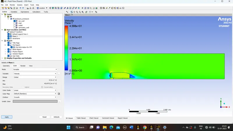
• Velocity Contour:
• 
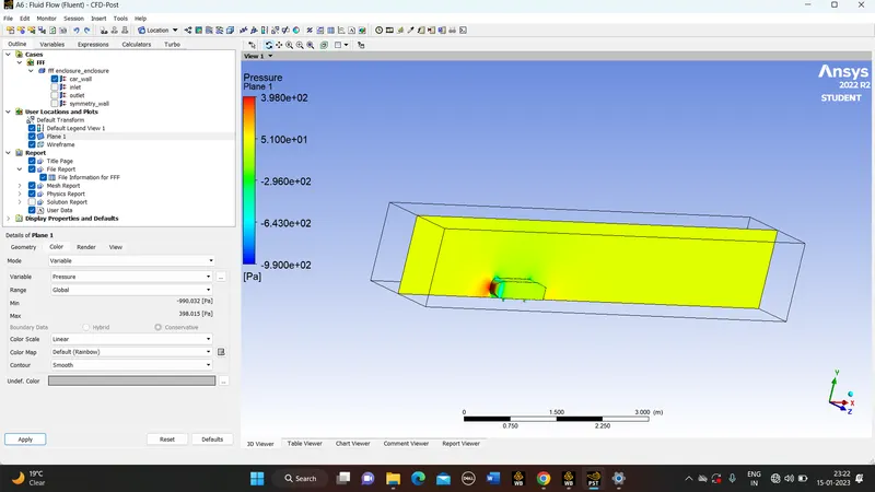
• Pressure Contour
• 
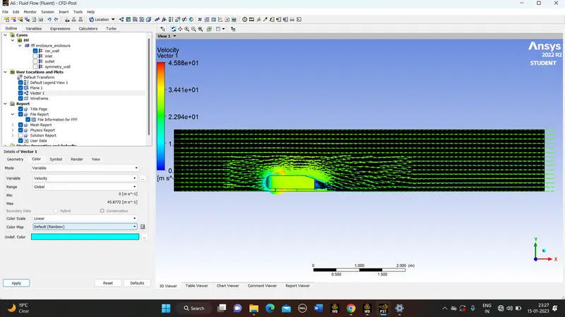
• velocity vector
• 
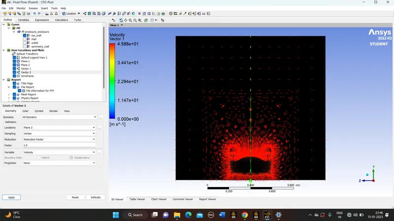
• velocity contour and vector in the YZ plane at varying distances from the plane
• 
• 
• 

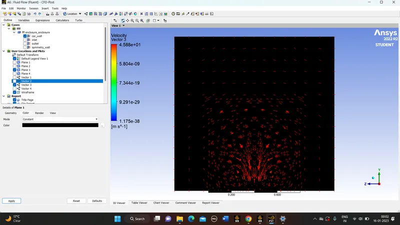
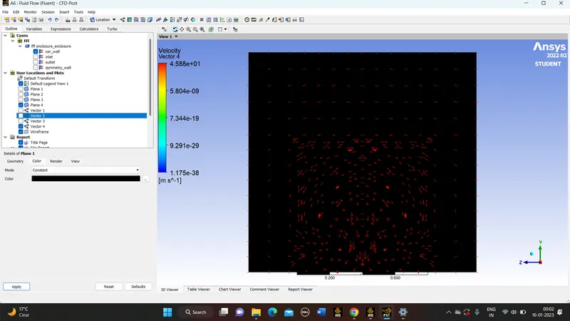
Velocity at 1.30

pThe following is the cause of the negative pressure that can be experienced in the wake region:

When approaching steep bends and turns, the flow of traffic tends to naturally split up, which is something that can be easily understood according to the principle of conservation of momentum.At the corner, the boundary layer keeps its momentum in the direction that the flow is going, and it is simply impossible for it to remain attached if there is not an external pressure gradient that is compelling it to turn around the corner.Therefore, because the flow has a tendency to proceed in a straight line, a low pressure region is formed at that point and at the back of Ahmed's body as a result of this.The flow that is moving in a straight line is then sucked in by the low pressure, which results in the formation of a recirculation zone and a big wake on the backside of the Ahmed body.In addition to this, a big wake is produced as a result.

If you look at the velocity contour, you can see where the wake is forming, and if you look at the pressure contour in the wake zone, you will see that there is a negative pressure.In point of fact, it is not the zone of negative pressure; rather, it is the region of low pressure.You are able to notice the negative values since we have taken our readings with reference to 0 gauge pressure.If you alter the outlet gauge pressure or run the simulation by taking absolute pressure, you won't get any negative readings, but you will get rounded-off errors because the flow can't be compressed, thus there will be slight changes in pressure.For this reason, it is recommended that simulations of incompressible flow use 0 gauge as their point of reference.

CONCLUSION

There is evidence to suggest that grid independence tests converge more rapidly for cells of smaller sizes.he drag and lift coefficients both decrease with decreasing mesh size.In calculating the magnitude of drag, Y+ is crucial.Since there is no flow in the wake zone, the pressure and velocity there are negative. Separation and recirculation are just two of the many possible explanations for this. It may be seen clearly in the vector plot around the wake Beyond the point of separation at the vehicle's tail end, the flow is seen to recirculate and attach itself to the boundary layer, marking the separation.When the mesh size is decreased, finer features of the vector indiacators can be seen in the plot.

THANK YOU