Week 3 - External flow simulation over an Ahmed body.

Aim:

1. Describe Ahmed body and its importance.
2. Simulate a flow over Ahmed body.
3. Plot the results and provide a conclusion for the obtained results.
4. Obtain the plot for drag coefficient.

Theory:

The Ahmed Body was first created by S.R. Ahmed in his research “Some Salient Features of the Time-Averaged Ground Vehicle Wake” in 1984. Since then, it has become a benchmark for aerodynamic simulation tools.

A layout of Ahmed Body along with its dimensions :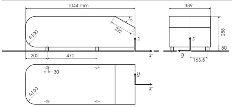



As shown in the figure it features a uniform rectangular cross section at the leading end while terminating with a slant at the trailing end defined using slant angle `phi`. The slant angle is kept around thee critical slant angle of 30 degrees (25 degrees to 35 degrees).The general flow field in wake region of ahmed body is shown below:

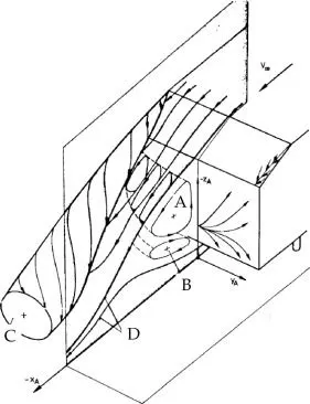
The Regions A & B are formed by flow seperation from top and bottom face of ahmed body respectively. These seperated flows create vortices in the wake region which are of opposite sense to each other. These formation of these regions are also responsible for maximum drag on the body which we will simulate and verify in this simulation.

Region C is formed when flow moves over top corner edges formed by top and side faces of the ahmed body.

Importance of Ahmed Body:

As the burning of fossil fuels becomes a more pressing issue, manufacturers are introducing more fuel efficient cars to the market. One main contributor to fuel burn is the car’s aerodynamic drag.Complex shaped cars are difficult to model and compute the aerodynamic drag computationally. So it would be really expensive and time consuming to validate the simulation tools over such complex models. What is rather done is, simulation tools are validated over Ahmed Body. The model is simple to model while maintaining car-like geometry features.

Simulation:

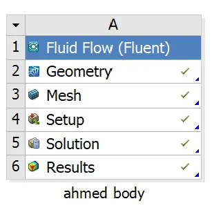
1. Create a standalone case from ToolBox over to Project schematic window.
   
2. Open Geometry in Space Claim and import the Ahmed Body model.
   
   
   
   
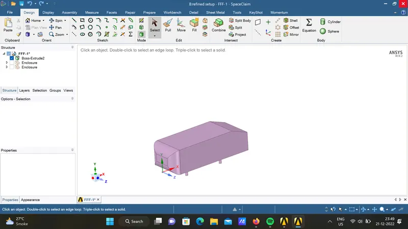
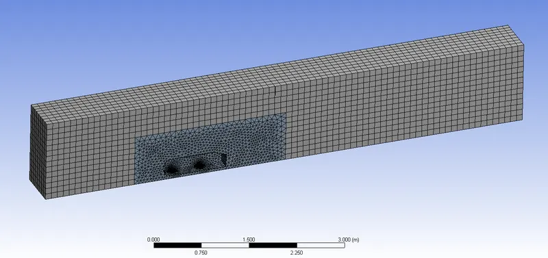
3. We define an enclosure around the ahmed body as our domain and also remove the interfering boundaries between the enclosure and the geometry.
   
   
   
   
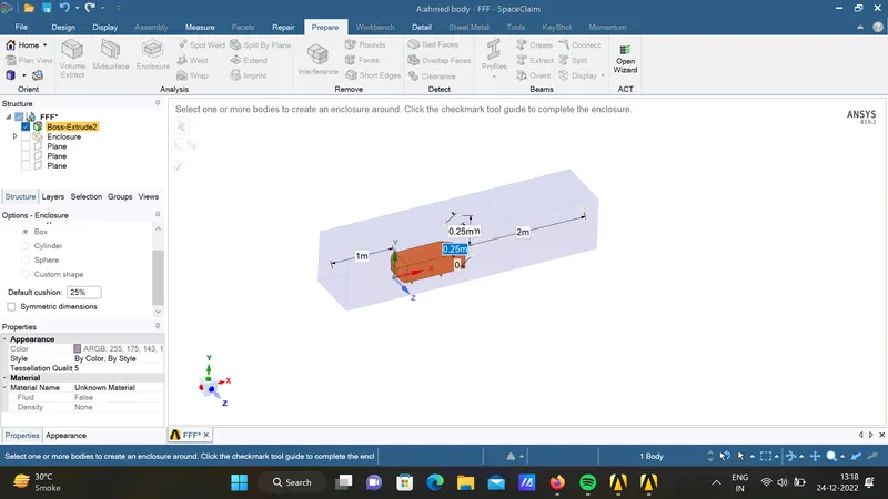
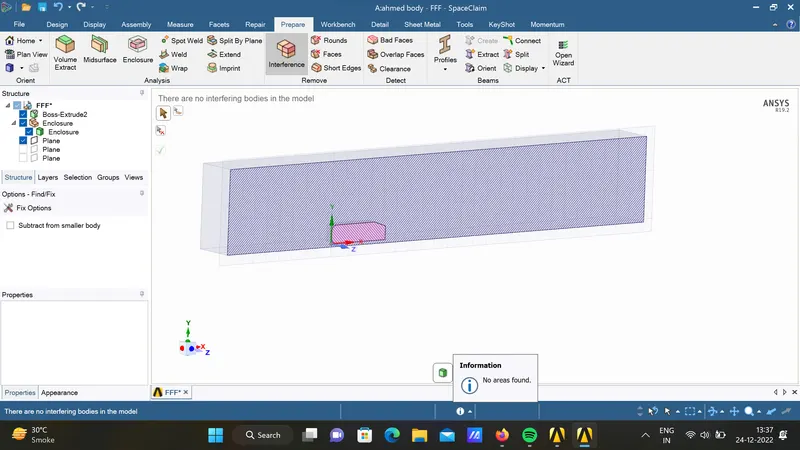
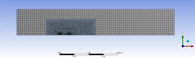
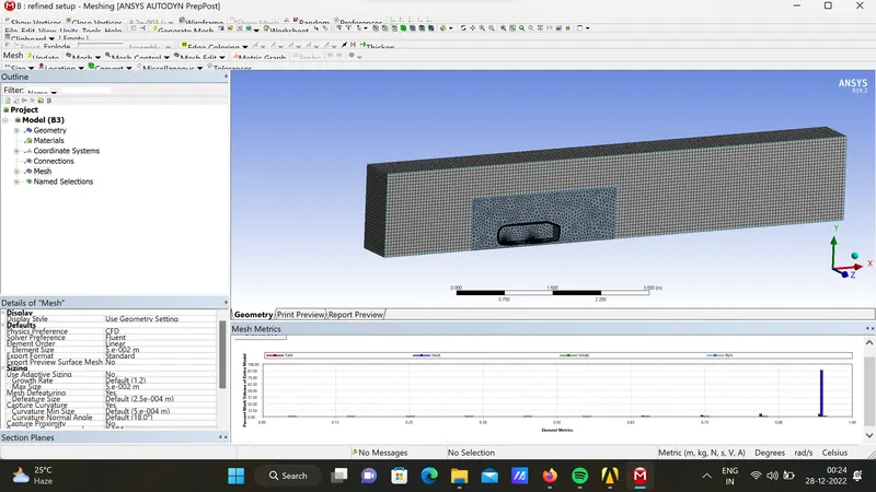
4. It is better if we define another smaller enclosure where we can have a mesh that is finer and also follows the geometry more closely for better results, and have a structured mesh in outer enclosure. This will help us with saving some computational time and efforts. Also as the body is symmetric in X-Y palne we can split the body using the 'Split Body' option under 'Design' tab to further reduce the computaional time.
   
   
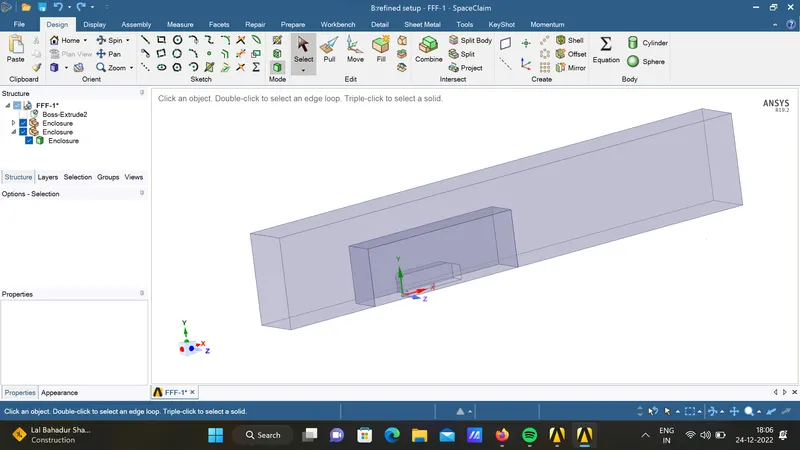
5. Boundary conditions are defined using named selection.
6. Load Mesh from the Project Schematic window.
   
   
   
   
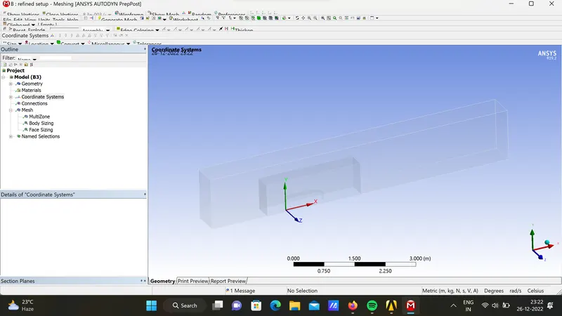
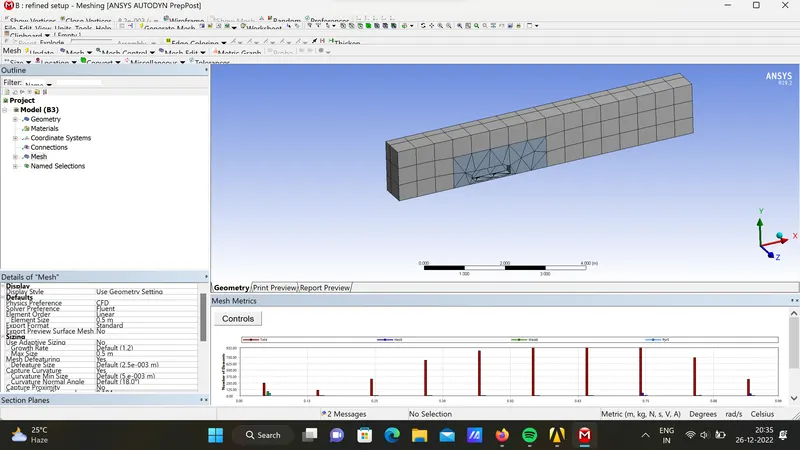
7. We choose different meshing techniques for different enclosures of the geometry.
   
   a) For the outermost enclosure we use multizone method under meshing option. The MultiZone mesh method provides automatic decomposition of geometry into mapped (structured/sweepable) regions and free (unstructured) regions. It automatically generates a pure hexahedral mesh where possible and then fills the more difficult to capture regions with unstructured mesh.
   
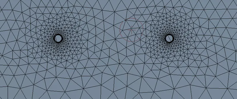
   b) For enclosure nearer to ahmed body we choose a finer mesh. We do it by choosing body sizing method which is essentially used to have a better control over the meshing in desired region. This overwrites the global mesh settings.
   
   c) For circular regions like the leg region we use face control to match the geometry more acurately. It is similar to body sizing but only for faces.
   
   
   
   
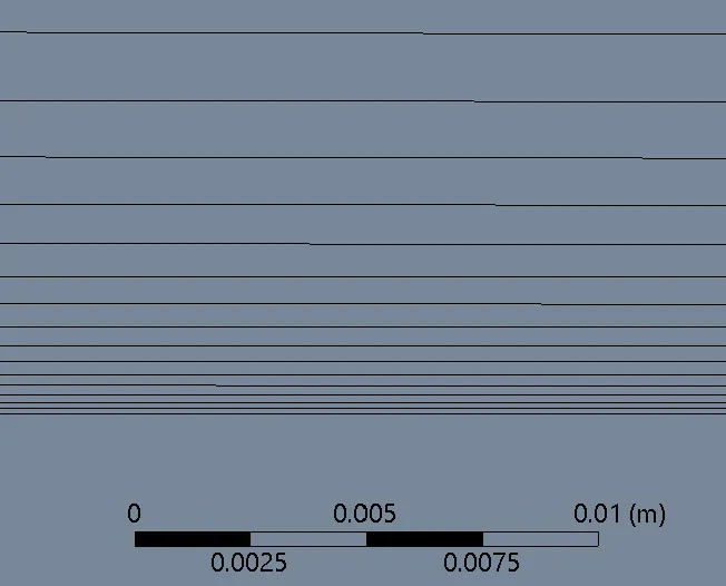
8. But to capture the wall effects the elements should match the geometry contour more closely. For that we use Inflation Layers.
   
   
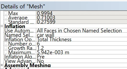
   We opted for Total Thickness Inflation Option. In this we define the cumulative thickness of the inflation layers. Since growth rate is 1.2, if we know the thickness of first layer then we can calculate the total thickness.
   
   How to we decide on what value to take for first layer thickness?
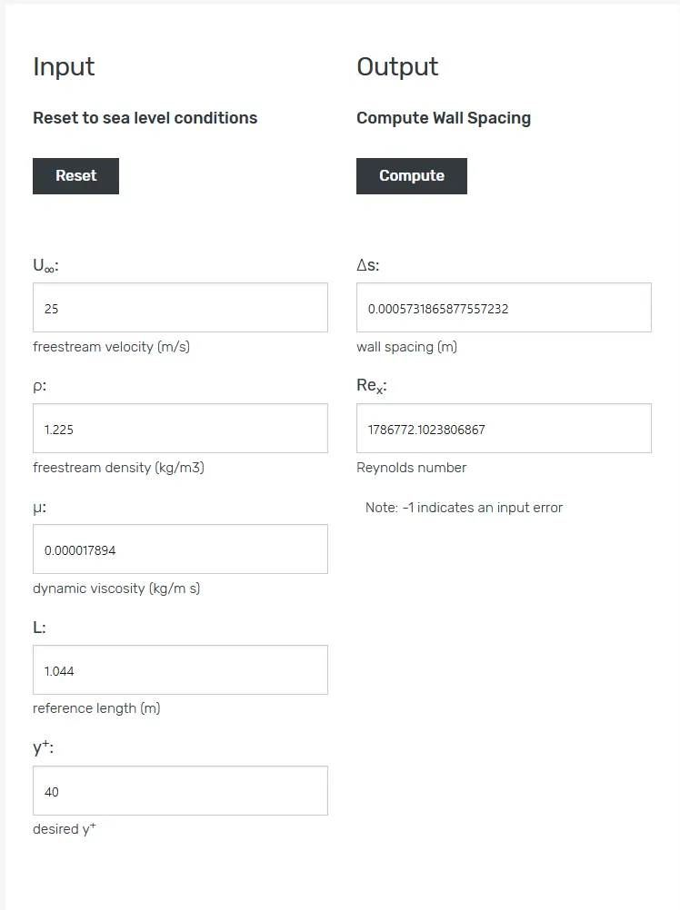
   We use the y+ value and we may use the y+ calculator for finding the thickness of first inflation layer.
   
   

   What is y+?

   y+ is the non dimensionalised wall thickness defined as `y^+=(y.rho.u_**)/mu` where,
   y is the wall distance, `u_**` is the friction velocity, `rho` is the density of the fluid and `mu` is the dynamic viscosity of the fluid.

   `k-epsilon` model works well for y+>30 values and it doesn't give accurate results for y+<30 values and would need wall functions or refined version of the model to solve for accurate near the wall simulations.
   

   The wall function is used to connect fluid flow in the near-wall region with fully developed turbulent flow. This method also helps reduce elements in the wall region, assisting in reducing computation time. The boundary layer is usually meshed with prism shape cells to capture the boundary layer and its viscous sublayer effectively. In CFD solvers, this method is often known as inflation layer meshing. Inflation layers makes elements appear as an extention of the geometry by replicating the geometry contour in order to accurately simulate the flow near the walls.
   
   
   
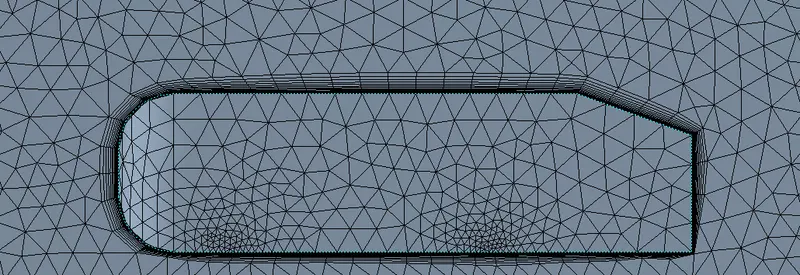
   The first point from the wall from where `k-epsilon`is aplicable in ansys fluent is represented by first layer thickness of inflation layer. This can be obtained from one of the many available calculators online. Like the one mentioned in the reference reaction.
   
   

   How y+ calculator works:

   It takes values for reference length, free stream velocity, density and viscosity values of the fluid. Using these values Reynolds Number is calculated and from one of the emperical relations for coefficent of friction (example like Prandtl's Relation `0.074 Re_x^(-0.2)`).

   The wall shear stress is calculated using relation `tau_w=1/2C_f rhoU_f^2`.

   Using relation between shear velocity and shear stress `u_**=sqrt(tau_w/rho)`, shear velocity `'tau_w'` is computed.

   Putting all these values in y+ equation, y is calculate which is used as First layer thickness of inflation layer.
   
   
   
   The mesh quality was also satisfactory.
   
   
   

9. We close the Meshing window and run the fluent setup from project schematic.
   
   
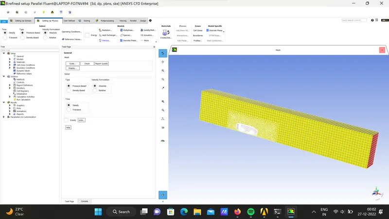
   Steady, Pressure based solver is chosen as flow is considered incompressible (Ma<0.3). Therfore no density based solver and hence energy equation is not used.
   Viscous `k-epsilon`turbulence model is used.
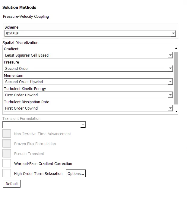
   SIMPLE algortihm with least square cell based space descritization is used.
   
   
   
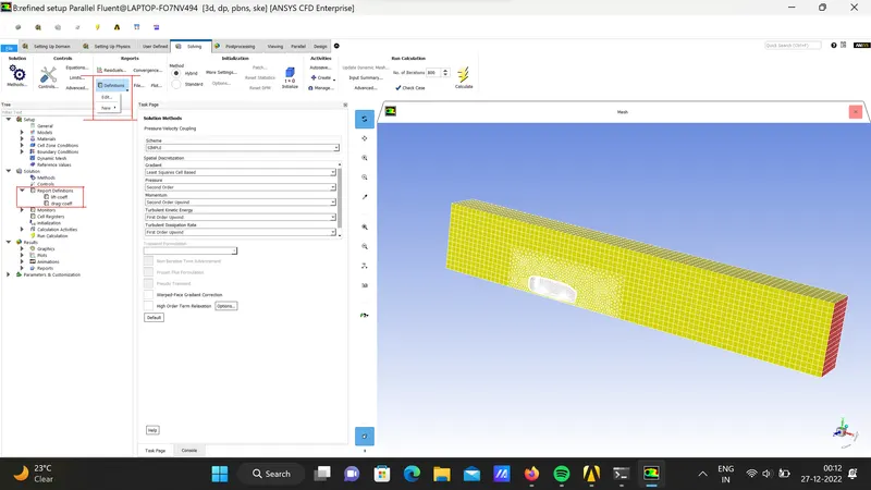
10. Report definitions are created for coefficient of drag and coefficient of lift.
    
    
    
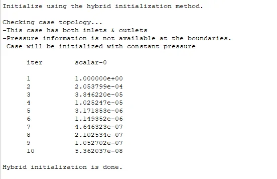
11. Hybrid Initialization is used to initialize the solution.
    
    
12. In post processing section we define contour plots for velocity and pressure. Followed by running the simulation for a given number of iterations.
    

Results:
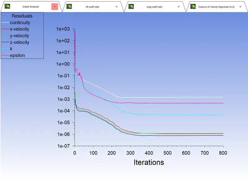
The meshing and simulation was done for maximum element sizes of 0.5, 0.3, 0.2 and 0.1. The results obtained are as follows:

1. Maxiumum Mesh Element Size of 0.5m
   
   
   
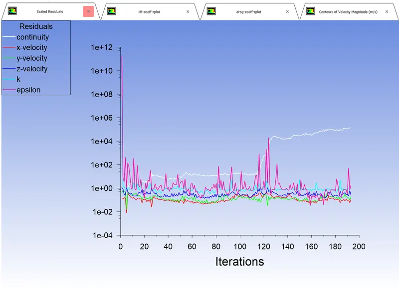
   The resuiduals didnt achieved stability instead continuity residuals goes on increasing. Hence mesh refinement was done.
   
2. Maximum Mesh Element Size of 0.3m
   
   
   
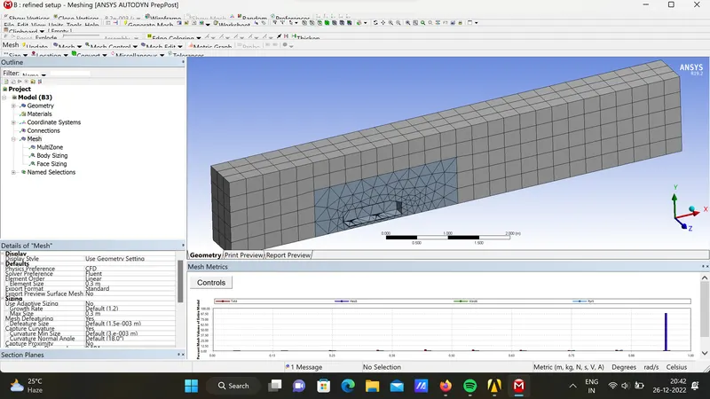
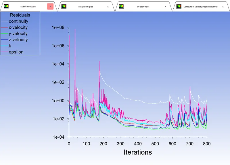
   Again residuals dont show any sign of stabilty. Further refinement of mesh was done.
   
3. Maximum Mesh Size of 0.2m
   
   
   
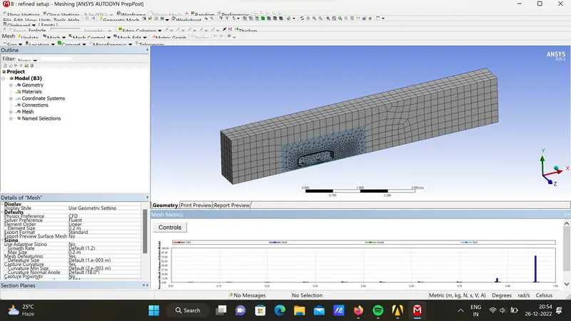
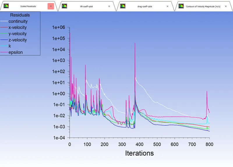
   Though still unstable residual plot is still better than previous cases, suggesting further refinement of mesh might lead to stability.
   
4. Maximum Mesh Size of 0.1m
   
   
   
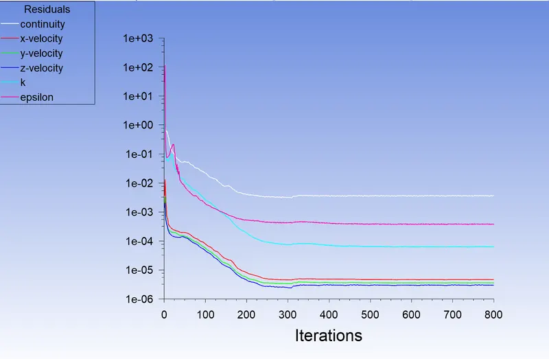
   The Residual plot shows stability is achieved.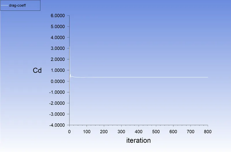
   
   
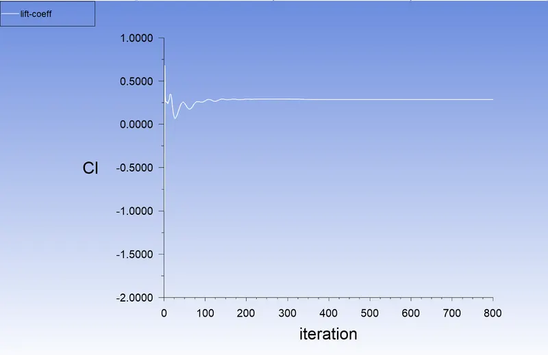
   coefficient of drag coefficient of lift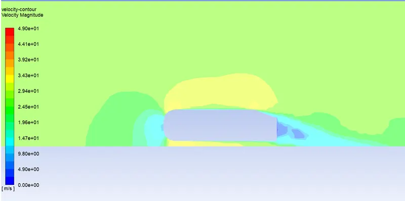
   
   
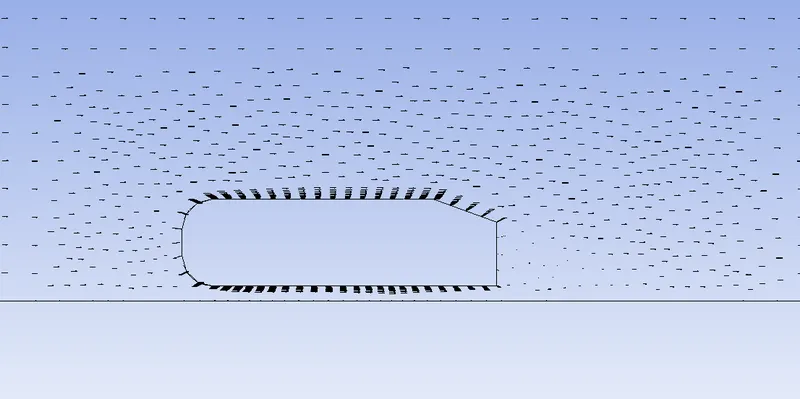
   velocity contour plot veelocity vector plot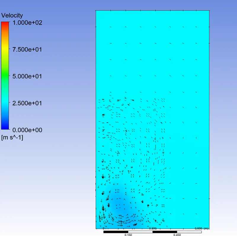
   
   
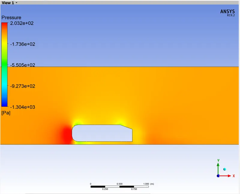
   Velocity Vector plot across the ahmed body in wake region Pressure Contour Plot
   
   
   
   Coefficient of drag was found out to be 0.3612.
   
   
5. Maximum Mesh Size of 0.05m
   
   
   
   
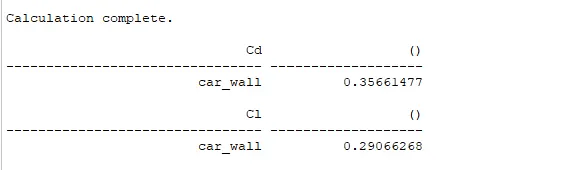
   Coefficient of drag was found out to be 0.35
   
   The scaled residues achieved stability and results are similar to the case of maximum mesh size of 0.1m. This shows that grid independency is achieved.
   
   
6. A case was also simulated with Maximum Mesh Size of 0.1 m and flow velocity of 50 m/s.
   
   
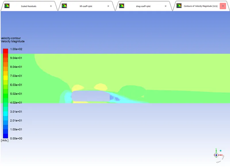
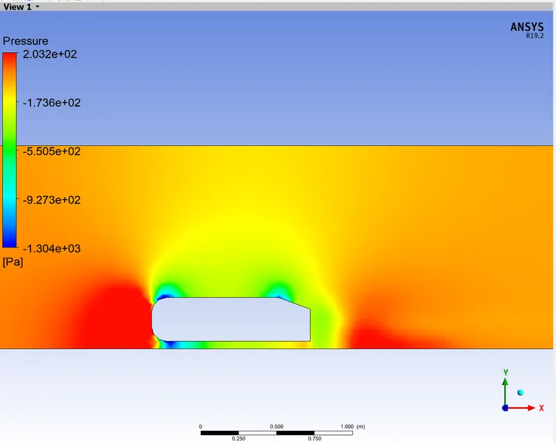
   velocity contour plot pressure contour plot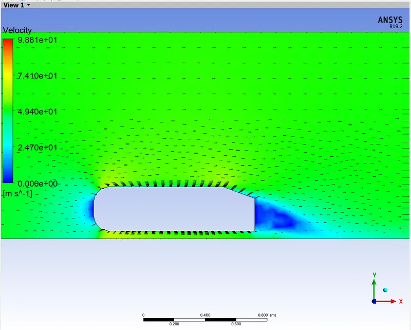
   
   
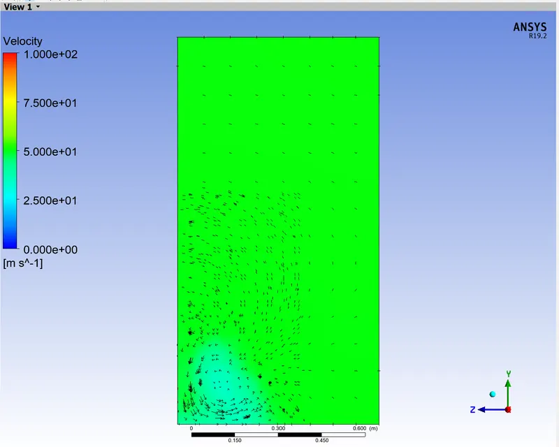
   velocity vector plot Velocity Vector plot across the ahmed body in wake region
   
   
   Coefficient of drag was found out to be 1.4302.
   With an increase in flow velocity the drag coefficient also increased.

Conclusion:

1. From Velocity contour plots we see a low velocity region in the wake of the ahmed body. This low velocity wake region are characterized by formation of vortices after flow seperation. What can be inferred from it is there is a reverse pressure gradient that makes the flow rotate back towards the body at the wake region.
2. As evident from velocity-vector plot the flow is attached to the boundary of ahmed body till the slant face at the rear.
3. The Pressure contour plot shows the pressure is maximum at the nose end of the body as the kinetic energy is converted to pressure and the pressure there is known as Stagnation Pressure.
4. The Pressure in the wake region is lower than at the nose. this pressure difference creates a pressure drag which further increases the drag coefficient of the body.
5. When velocity of the flow is increased drag coefficient was also increased. This is because High-Reynolds Number Flow causes the flow to seperate early and meet farther away in the wake region which increases the Adverse Pressure Grradient and is the cause for a negative pressure in the wake region sometimes.

References:

1. https://www.comsol.com/blogs/studying-the-airflow-over-a-car-using-an-ahmed-body/
2. https://www.cadence.com/ko_KR/home/tools/system-analysis/computational-fluid-dynamics/y-plus.html
3. https://www.omnicalculator.com/physics/yplus
4. https://www.simscale.com/forum/t/y-yplus-generate-wall-spacing-for-cfd/82451