Week 3 - External flow simulation over an Ahmed body.

AIM: External flow simulation over an Ahmed body.

Expected result:

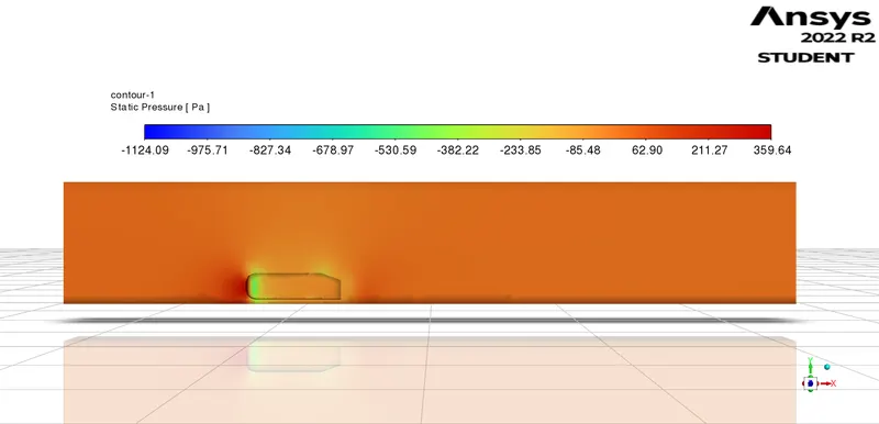
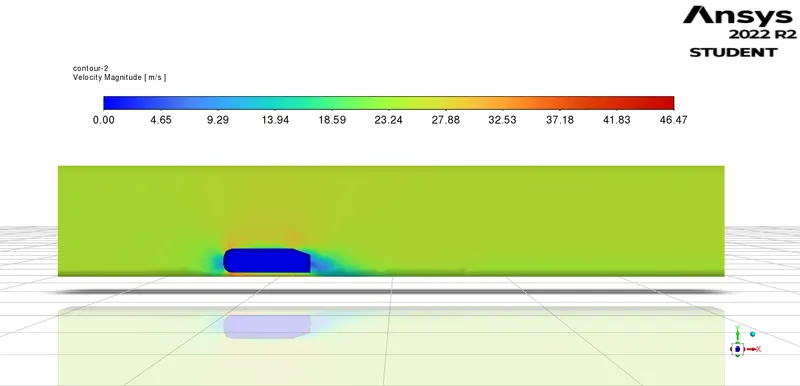
1. Velocity and pressure contour.
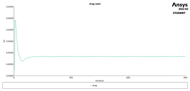
2. The drag coefficient plot for the refined case.
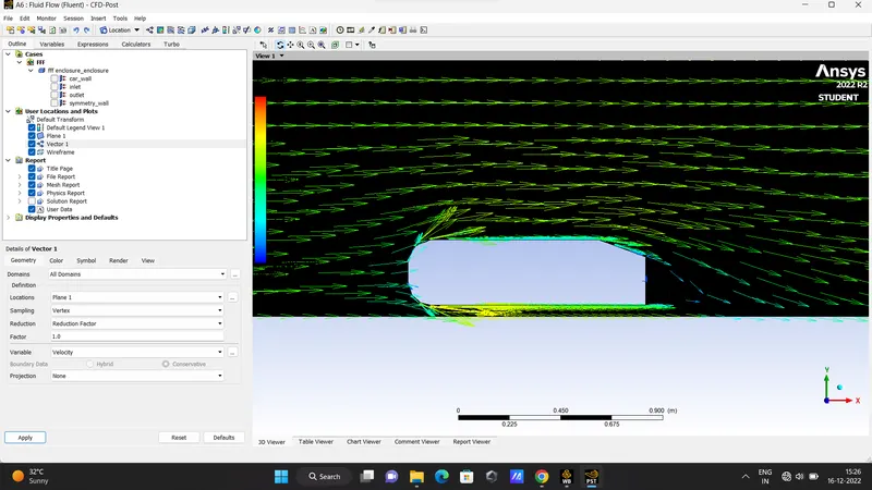
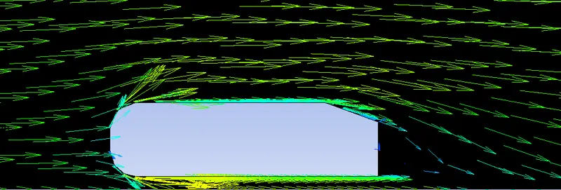
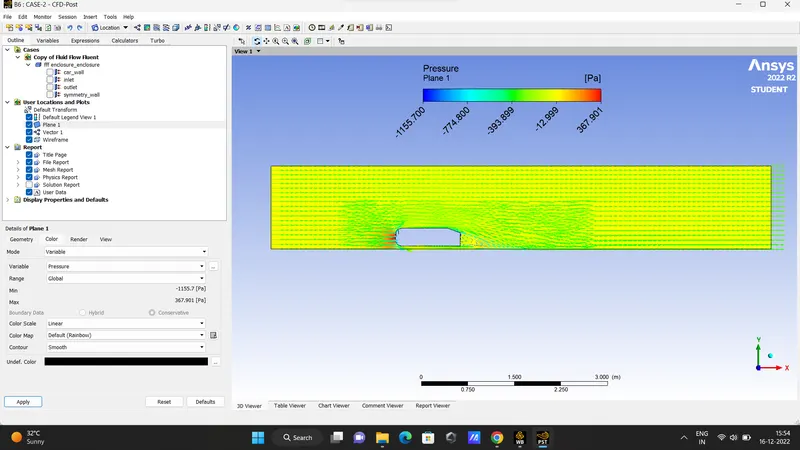
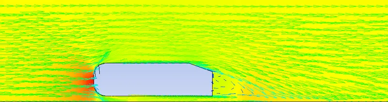
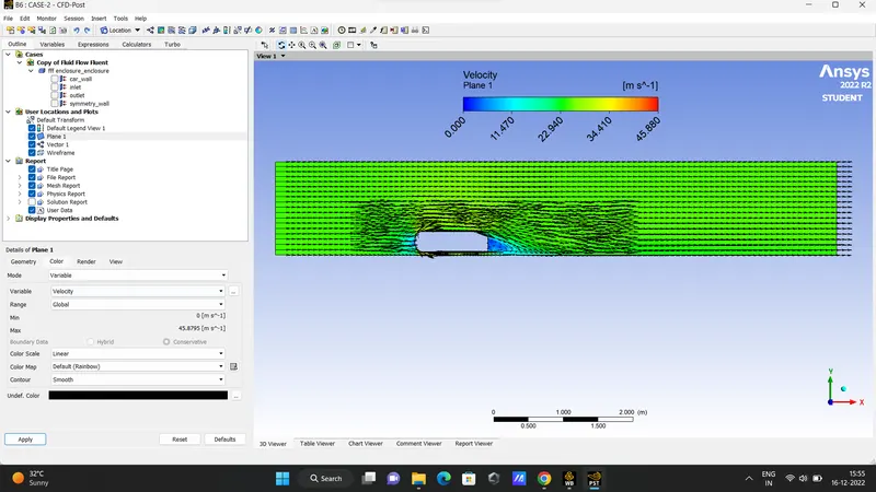
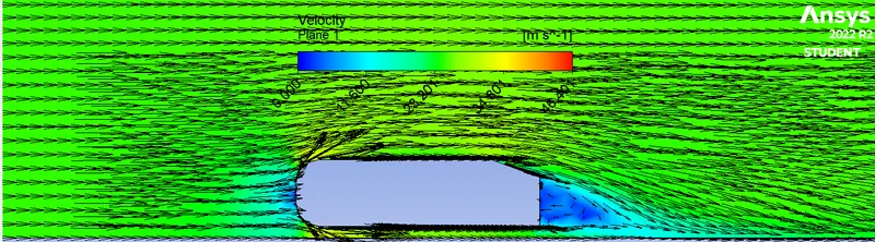
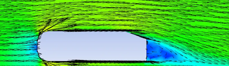
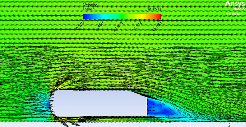
3. The vector plot shows the wake region.
4. Provide drag and lift coefficient values for each case.

Given data:

The flow velocity of air = 25 m/sec.

Theory:

The Ahmed body is a generic car body (a simplified vehicle model). The airflow around Ahmed body captured the essential flow features around an automobile like wake forces, drag forces, etc., and was first defined and characterized in 1984 by Ahmed et. al.

Although it has a square shape, Ahmed body allows us to capture characteristic features that are relevant to bodies in the automobile industry.

This model is also used to describe the turbulent flow field around a car-like geometry. Once the numerical model is invalidated, it is used to design new car models.

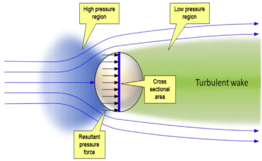
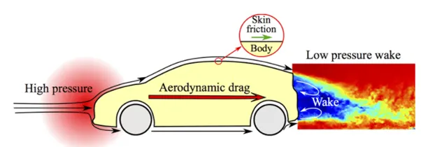
Negative pressure in the wake region and point of separation

Wake region:

Consider a fluid particle flows within the boundary layer around the circular cylinder. From the pressure distribution measured, the pressure is maximum at the stagnation point and gradually decreases along the front half of the cylinder. the flow stays attached to this favorable pressure reason as expected. However, the pressure starts to increase in the rear half of the cylinder and the particles now experience an adverse pressure gradient. consequently, the flow separates from the surface. It creates a highly turbulent region behind the cylinder called ‘Wake’. the pressure inside the wake region remains low as the flow separates and a net pressure force(pressure drag) is produced.

Procedure:

• Import Ahmed body geometry in SpaceClaim.

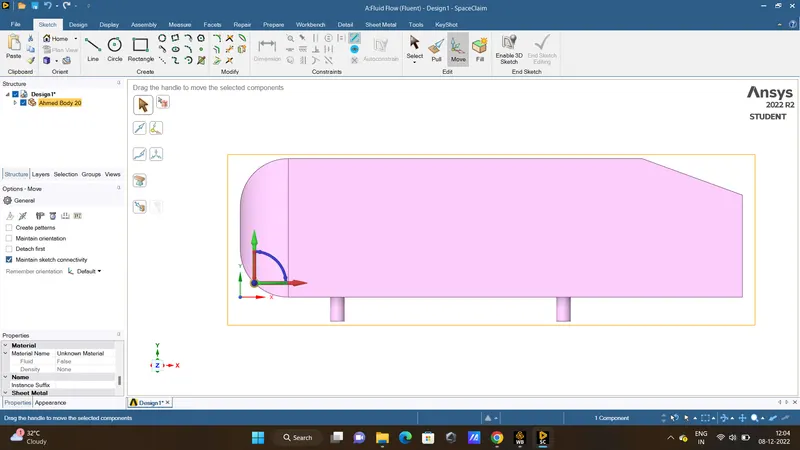
• Prepare an Enclosure for the Ahmed body

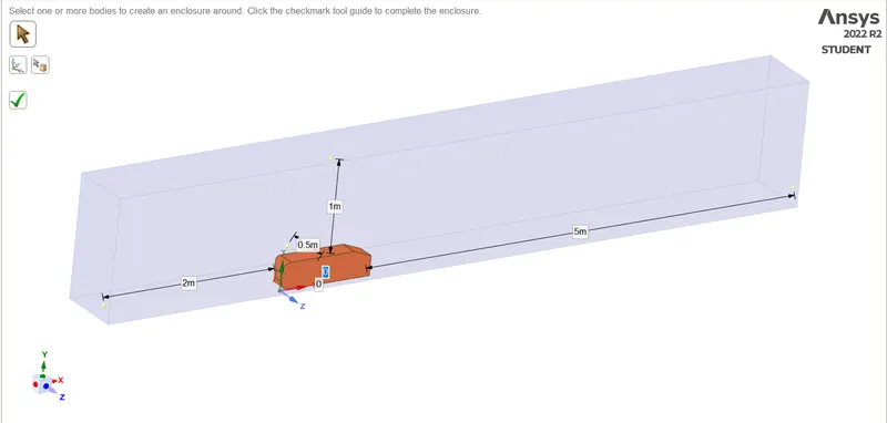
• Add another Enclosure of smaller dimensions.

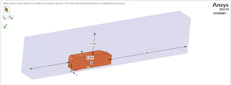
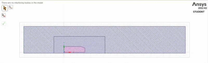
The final geometry after adding Enclosures is shown below:

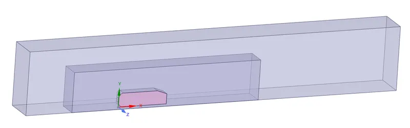
• Add a plane and view in section mode for interference.

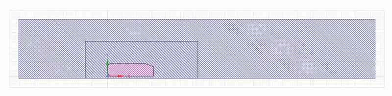
• In prepare section click on interference, it will show the interference region.

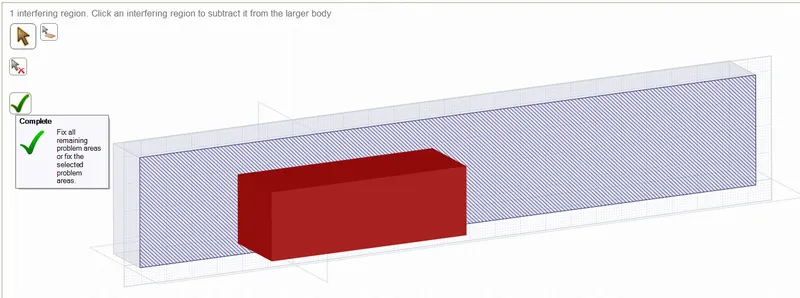
• Press on the green tick and It will resolve the interference problem.

• Suppress Ahmed body for physics.

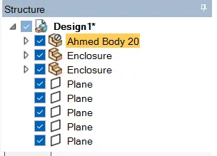
• Close SpaceClaim.

Meshing

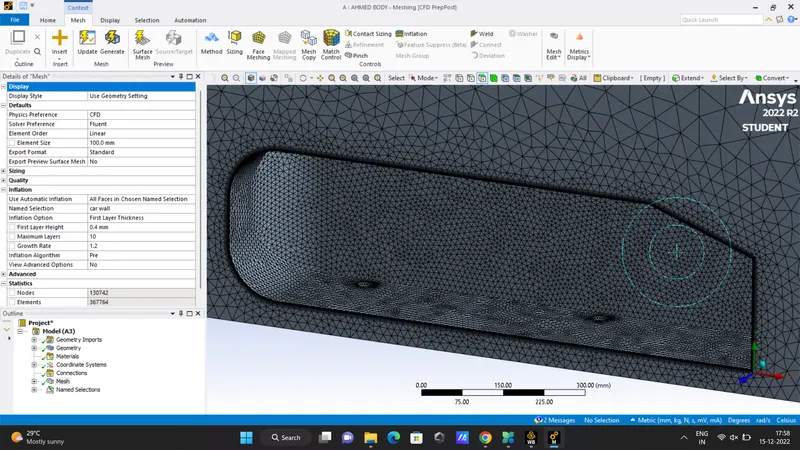
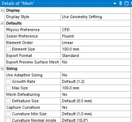
• Open the meshing interface and click on generate mesh at default values.

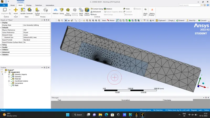
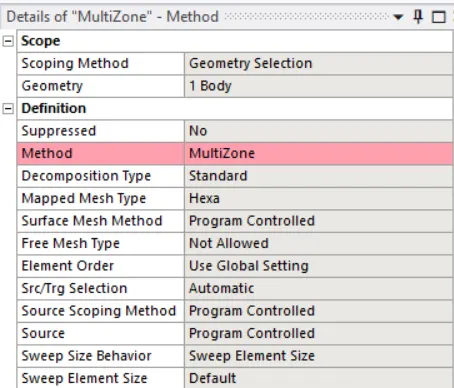
• Now insert a meshing method and for the method used multizone. When we use multizone it will automatically use hexahedral mesh where ever possible.

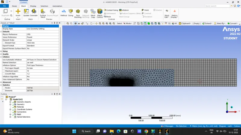
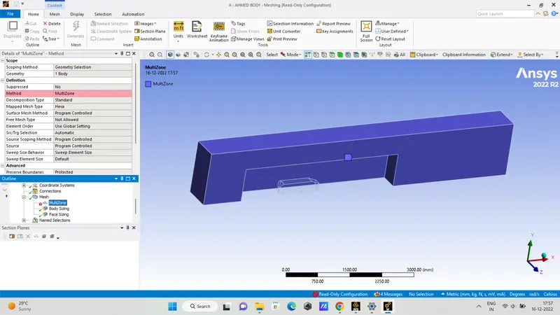
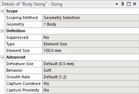
• Now insert sizing and select the inner box as geometry and element size as per requirement and generate the mesh.

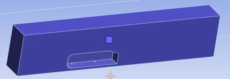
• Insert sizing and select 2 cylindrical stands of the body for the geometry and apply and set element size as per requirement.

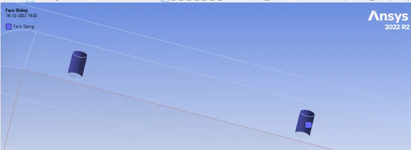
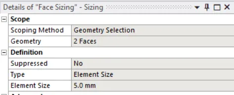
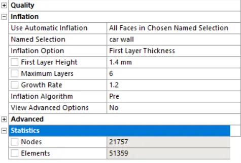
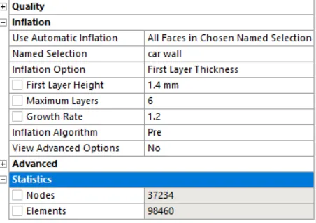
• Add the inflation layer to the car-body surface and select the inflation option as the first layer thickness.
  • First layer height as calculated from Y_p.
  • Maximum layers = 6
  • Growth rate = 1.2

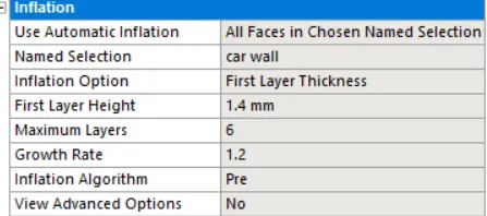
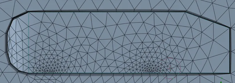
Inflation layers:

close meshing.

SETUP

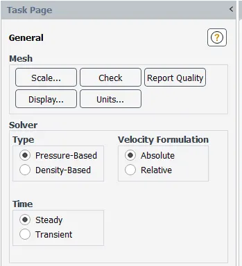
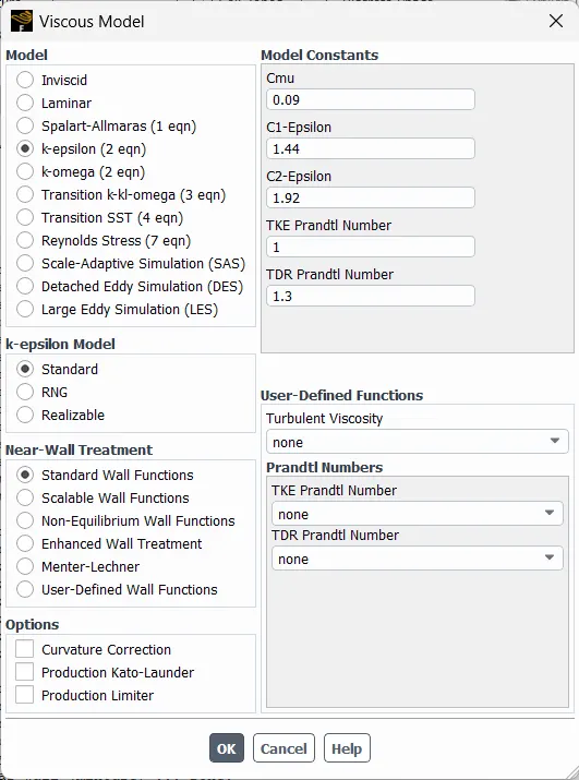
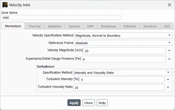
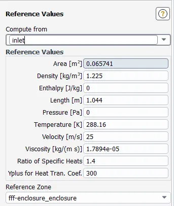
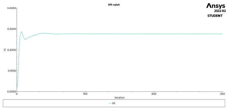
Create a definition for the drag coefficient and lift coefficient.

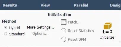
then INITIALIZE (HYBRID)

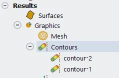
After Initialization creates PRESSURE CONTOUR & VELOCITY CONTOUR plots.

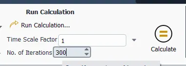
• Run calculation

DONE.

=====================================================================================================================================================

Output from the simulation

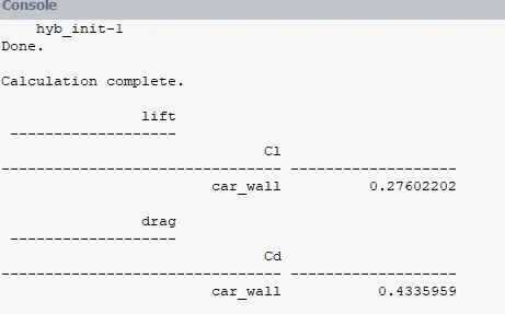
Case – 1

For bigger Enclosure

Mesh element size = 100mm

Maximum size = 100mm

Inflation (car wall) no. of layers = 6

Growth rate = 1.2

Inflation option = first layer thickness

First layer thickness = 1.4mm

For smaller Enclosure

Body sizing

Element size = 100mm

Face sizing bottom leg

Element size = 5mm

No. of nodes = 21757

No. of elements = 51359

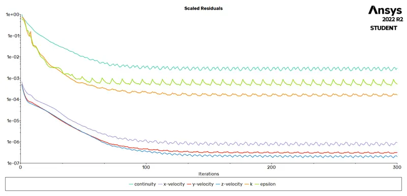
Residuals

Coefficient of lift

Coefficient of drag

Pressure contour

Velocity contour

Vector plot

-------------------------------------------------------------------------------------------------------------------------------------

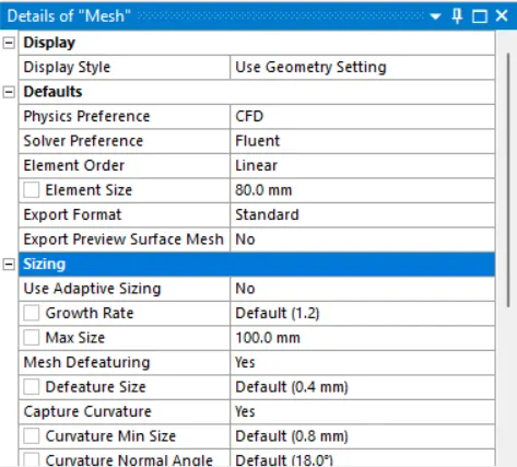
Case – 2

For bigger Enclosure

Mesh element size = 80mm

Maximum size = 100mm

Inflation (car wall) no. of layers = 6

Growth rate = 1.2

Inflation option = first layer thickness

First layer thickness = 1.4mm

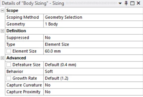
For smaller Enclosure

Body sizing

Element size = 60mm

Face sizing bottom leg

Element size = 5mm

No. of nodes = 37234

No. of elements = 98460

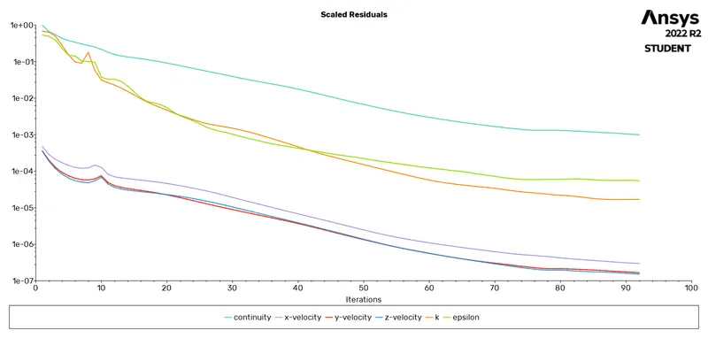
Residuals

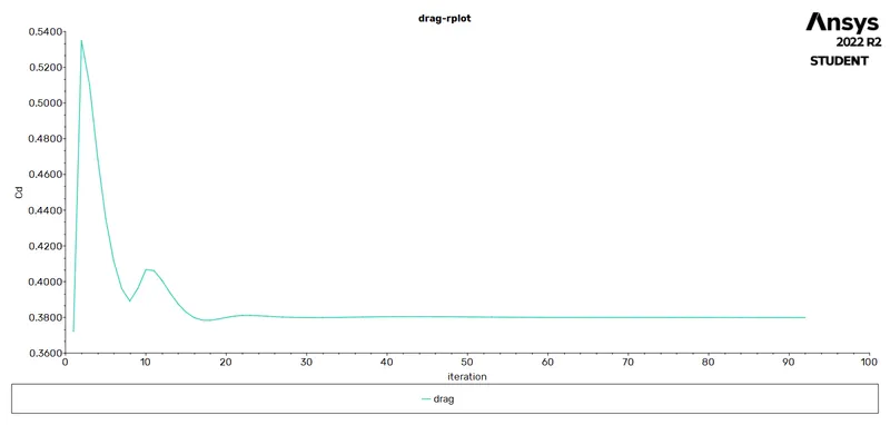
Coefficient of drag

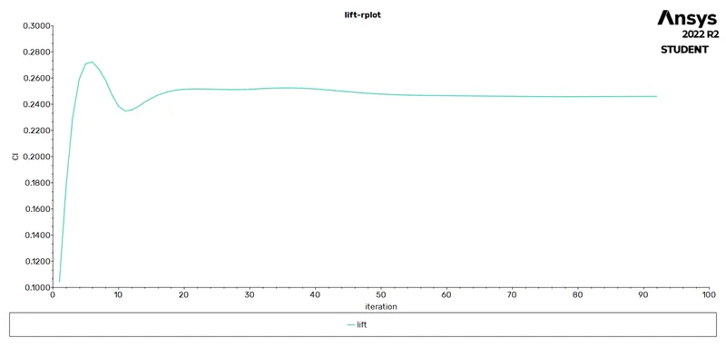
Coefficient of lift

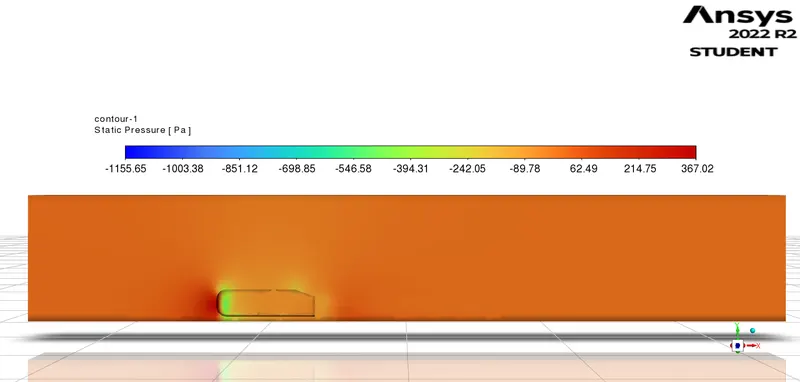
Pressure contour

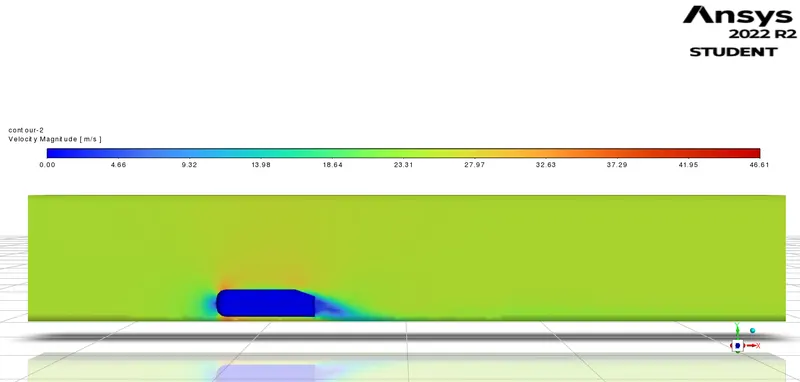
velocity contour

Vector plot

======================================================================

Case – 3

For bigger Enclosure

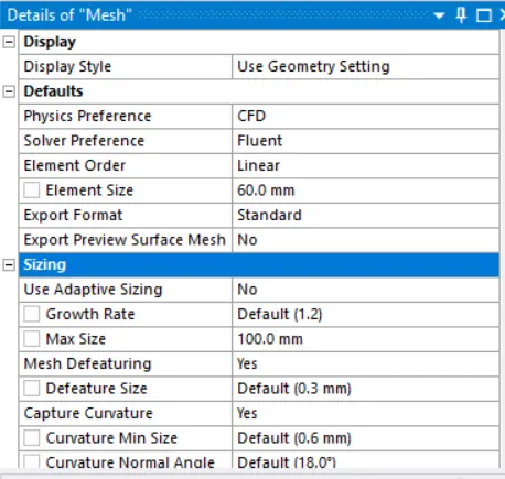
Mesh element size = 60mm

Maximum size = 100mm

Inflation (car wall) no. of layers = 6

Growth rate = 1.2

Inflation option = first layer thickness

First layer thickness = 1.4mm

For smaller Enclosure

Body sizing

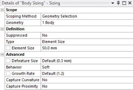
Element size = 50mm

Face sizing bottom leg

Element size = 5mm

No. of nodes = 63049

No. of elements = 156058

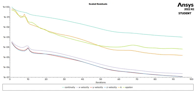
Residual

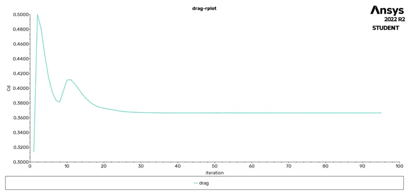
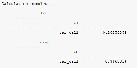
Coefficient of drag

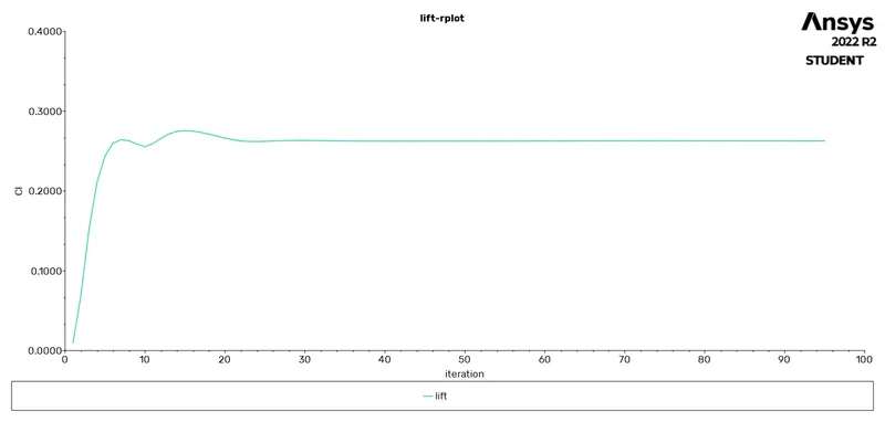
Coefficient of lift

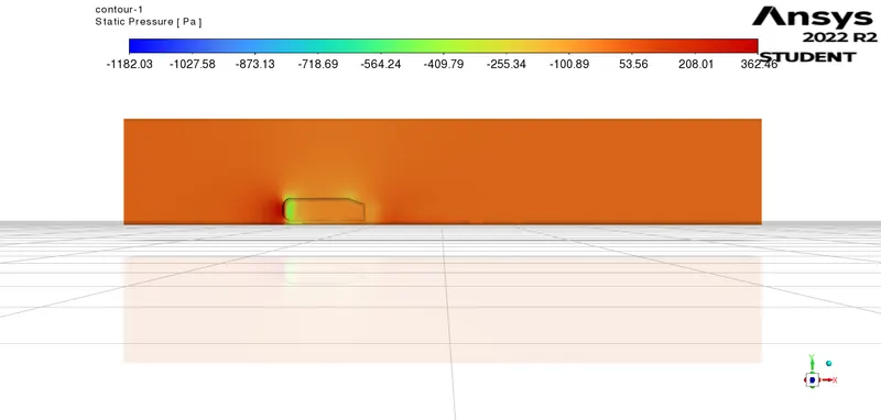
Pressure contour

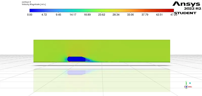
Velocity contour

Vector plot

==========================================================================

Case – 4

For bigger Enclosure

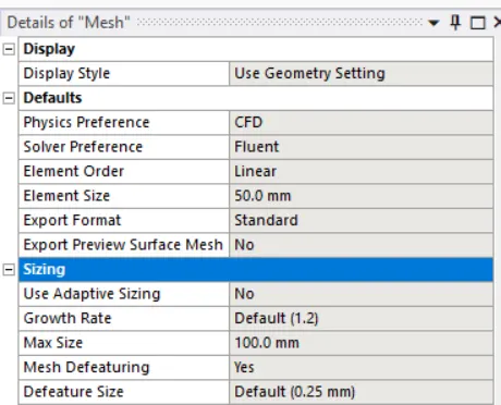
Mesh element size = 50mm

Maximum size = 100mm

Inflation (car wall) no. of layers = 6

Growth rate = 1.2

Inflation option = first layer thickness

First layer thickness = 1.4mm

For smaller Enclosure

Body sizing

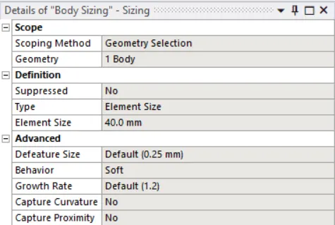
Element size = 40mm

Face sizing bottom leg

Element size = 5mm

No. of nodes = 99782

No. of elements = 263431

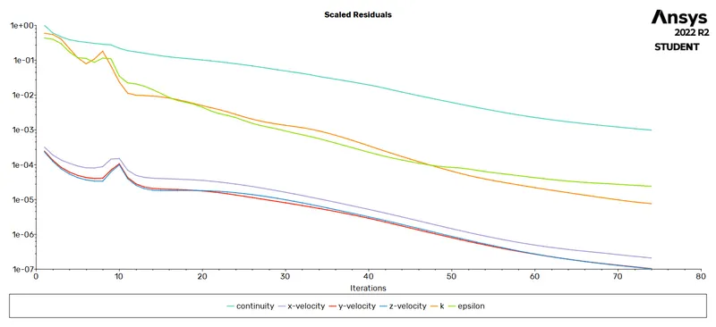
Residual

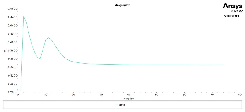
Coefficient of drag

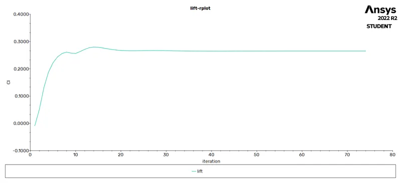
Coefficient of lift

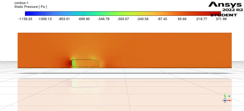
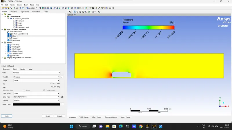
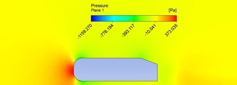
Pressure contour

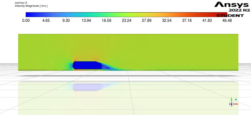
Velocity contour

Vector plot

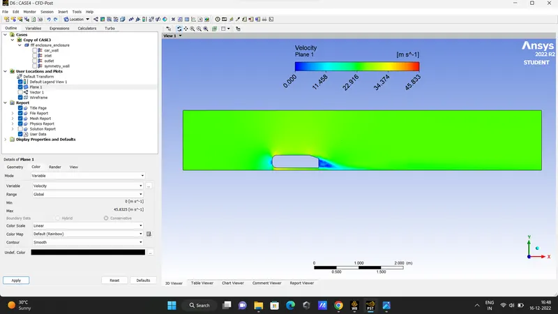
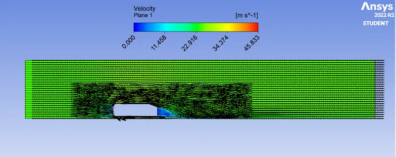
wake region

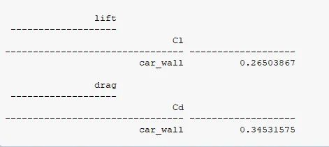
Comparison Table

Y+	YpYp (mm)	Outer box mesh size (mm)	Inner box mesh size (mm)	Drag coefficient	Lift coefficient
100	1.4	100	100	0.43359	0.27602
100	1.4	80	60	0.37988	0.24603
100	1.4	60	50	0.36653	0.26258
100	1.4	50	40	0.34531	0.26503

Conclusion

• We can observe that the value of the coefficient of drag is reducing and the coefficient of lift is increasing (except in the first case) as we are refining the grid size this is happening because we are refining near walls of the car body based on y + values.
• In the wake reason, we can see that there is a formation of a recirculation zone due to boundary layer separation at the back of the body.
• All the case studies were performed by considering the velocity of 25 m/sec. it is expected to see that an increase in velocity will cause boundary layer separation near the beginning of the slant surface and more vertex formation at the back of a body
• The study of static pressure contour helps us in understanding the sudden deceleration of flow and the red color indicates that static pressure raises the front of the body.