Week 3 - Solving second order ODEs

Aim : To write a program in Matlab that will simulate the simple pendulum motion.

Objective : To create a code for simple pendulum & create video for pendulum motion & displacement & find velocity.

ODE ( ordinary differential equation ) : An ODE is an equation containing an unknown function of one real or complex variable x. The unknown function is generally represented by a variable which depend on x.

second order differential equation for simple pendulum : The position of the bob with respect to time for the pendulum can be determined by using second order differential equation using matlab.

The 2nd order ode for simple pendulum will be as follows,

Description :

Given Data : g = 9.81m/s^2 % gravity in m/s^2

l = 1m % length of the pendulum in m

m = 1m % mass of the ball in kg

b = 0.05 % damping coefficient

angular velocity is the time rate at which an object rotates, or revolves, about an axis, or at which the angular displacement between two bodies changes.

here we have a angular velocity = 3 rad/sec at time t = 0

so we write code according it,

theta_0 = [0;3]

After that select time

time span is 0 to 20 sec & value 500 intervals

t_span = linspace(0,20,500)

after that we write differential equation ,

[t,result] = ode45(@(t,theta)ode_function(t,theta,b,g,l,m),t_span,theta_0)

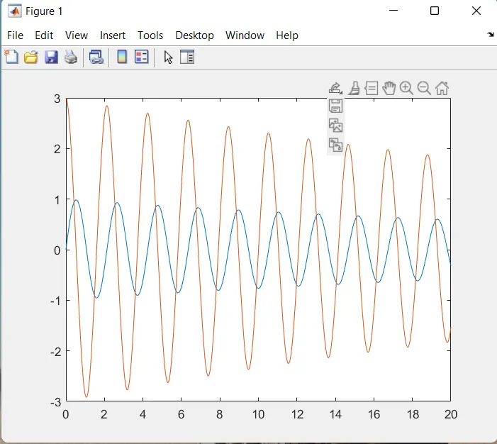
after that write code for plot damping & oscilation value

figure(1)

plot(t,result(:,1))

hold on

plot(t,result(:,2))

in fig. 1 shows a graph for value of damping & oscillation.

set the counter to the one

ct = 1

executing for loop from results of theta from linspace

for i = 1:length(result(:,1))

after that we select initial coordinates for pendulum

x0 = 0

y0 = 0

here always sert a 0 after that write a code for x & y position value .

formula for x1 & y1 position.

x1 = 1*sin(results(i,1)) for vertical

y1 = -1*cos(results(i,1)) for horizontal

y negative because pendulum downward position

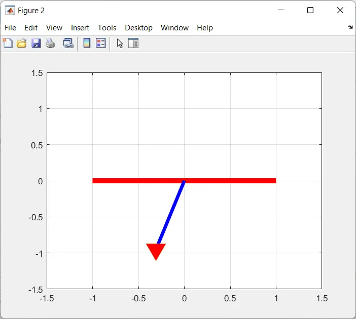
after that write code for pendulum movement

plot([-1 1],[0 0],'linewidth',6,'color','r')

hold on

line([x0 x1],[y0 y1],'linewidth',4,'color','b')

plot(x1,y1,'v','markers',20,'markerfacecolor','r')

hold off

grid on

axis([-1.5 1.5 -1.5 1.5]) define axis of graph

pause(0.005) value so animation of pendulum video

after that write code create animation of pendulum movement given below

M(ct) = getframe(gcf);

ct = ct+1; %incrementing counter

end

Animation video file code :

movie(M)

videofile = VideoWriter('ode_pendulum.avi','Uncompressed AVI');

open(videofile)

writeVideo(vidofile,M)

close(videofile)

Program Code :

clear all
close all
clc

% inputs
g = 9.81   % gravity in m/s^2
l = 1      % Length of the pendulum in m
m = 1      % mass of the ball in kg
b = 0.05   % damping coefficient

% define intial displacement & velocity
% given data - simple motion between 0-20 sec for angular displacement=0,
%angular velocity = 3 rad/sec at time t = 0,
theta_0 = [0;3];

% time input (given)
%time span is 0 to 20 seconds & get value 500 intervals
t_span = linspace(0,20,500);

% differential euqation
[t,results] = ode45(@(t,theta)ode_func(t,theta,b,g,l,m),t_span,theta_0); % ode solve one degree equation

% plotting the damping & oscillation values
figure(1)
plot(t,results(:,1));
hold on 
plot(t,results(:,2));

%set the counter to the one
ct = 1;
for i = 1:length(results(:,1)) % executing for loop from results of theta from linspace
    % initial coordinates for pendulum 
    x0 = 0;
    y0 = 0;
    % formula for next position x1 & y1 ( vertical & horizontal )
    x1 = l*sin(results(i,1)); % for vertical
    y1 = -1*cos(results(i,1)); % for horizontal
    
    
    % plotting of pendulum movement & moving & adding bob
    figure(2)
    plot([-1 1],[0 0],'linewidth',6,'color','r');
    hold on
    line([x0 x1],[y0 y1],'linewidth',4,'color','b');
    
    plot(x1,y1,'v','markers',20,'markerfacecolor','r');
    hold off
    grid on
    axis([-1.5 1.5 -1.5 1.5]); % defining axis of graph
    pause(0.005);
    
    % create animation of pendulum movement
    M(ct) = getframe(gcf);
    ct = ct+1; %incremeting counter
end

movie(M)
videofile = VideoWriter('ode_pendulum.avi','Uncompressed AVI');
open(videofile)
writeVideo(videofile,M)
close(videofile)

for solving the ODE we are providing the formulas by using function , so we write function code. And get value of theta 1 & theta 2 .

ODE Function :

% ode_function 
function[dtheta_dt]=ode_function(t,theta,b,g,l,m);

theta1=theta(1);
theta2=theta(2);
dtheta1_dt=theta2;
dtheta2_dt=-(b/m)*theta2-(g/l)*sin(theta1);
dtheta_dt=[dtheta1_dt;dtheta2_dt];
end

video link :

https://drive.google.com/file/d/1F9FA7-FB-uhBvufbyid5YtndKobgK3-s/view?usp=sharing

velocity & displacement graph :