Week 3 - External flow simulation over an Ahmed body.

Aim: External flow simulation over Ahmed Body.

Objectives: Simulate the flow over the Ahmed body and use air as the working fluid with velocity of 25 m/s.

Geometry:

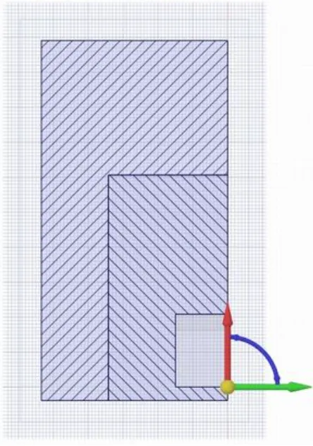
Enclosures are basically the flow fields. It is where the flow actually takes place. In this project, we create two enclosures, this is done to refine the area of study/interest or where the flow changes are highest.

Once this is done, always suppress the physics of the original geometry, as we will not require the mesh inside of the body. It is the surrounding area that is our focus.

Meshing:

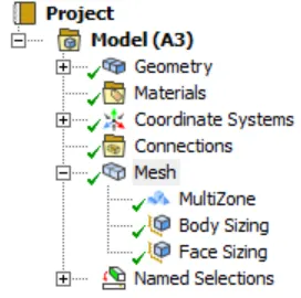
Method = Multizone
Effectivity = Outer Enclosure

This improves the uniformity and makes the mesh more structured. Also, reducing the number of cells, thus reducing the computational costs.

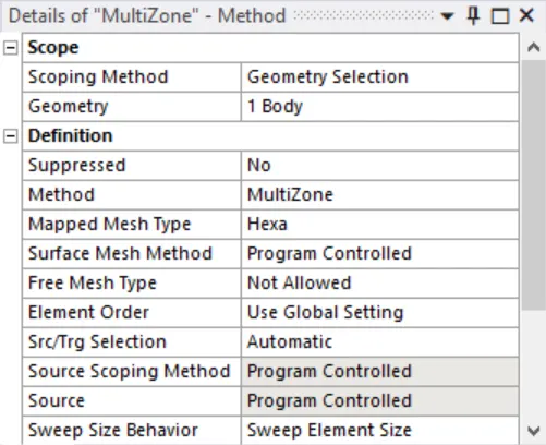
Method = Body sizing
Effectivity = Inner Enclosure

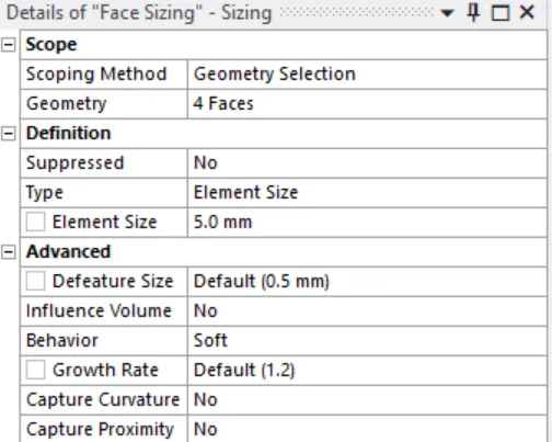
Method = Face sizing
Effectivity = Ahmed body

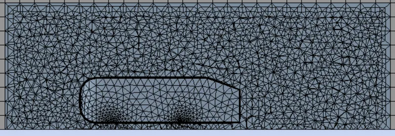
This is done hoping, that the cylindrical holes in the Ahmed body would get a circular boundary rather than the polygonal as shown in the following picture.

Setup:

Flow characterisitcs

Material = Air

ρ=1.225kgm−3ρ=1.225kgm-3

u=25ms−1

Since the Reynolds number is too high, we use the turbulent model.

• Pressure-based solver (Reason = Incompressible flow)
• Method = SIMPLE
• Steady flow
• Turbulent model
• Viscous = k-omega SST (Reason = Captures physics both at boundary layer and away from boundary layer)

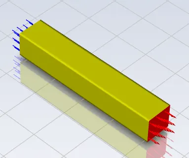
1. First, we need to check the mesh from Domain section.

2. secondly, check if the boundaries hve been specified correctly.

3. Now, provide the reference values according to the problem.

4. set the turbulence model (K-OMEGA (SST)).

5. Select the solver (simple taken by default setting) according to the problem.

6. Now, set in the boundary conditions like inlet velocity, guage pressure, etc.

Inlet velocity- 5 m/sec

outlet- gauge pressure = 0 pa

car wall- No sleep

7. In solution section create drag and lift reports and plots, also set the solution method.

8. Now, go to the results section and create a plane at some distance normal to x,y,z axis which will be used to examine the velocity and pressure along it.

9. Initialize the problem with Hybrid Initialization.

10. Go back to result section and add velocity and pressure contours along plane. Also add velocity animation.

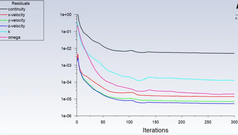
11. Finally simulate the problem for some amount of iteration and ovserve the Drag, Lift and Residual plots.

12. This completes the setup section.

Results:

Residual:

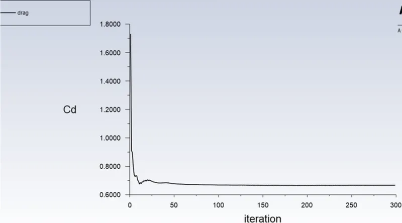
Drag co-efficient:

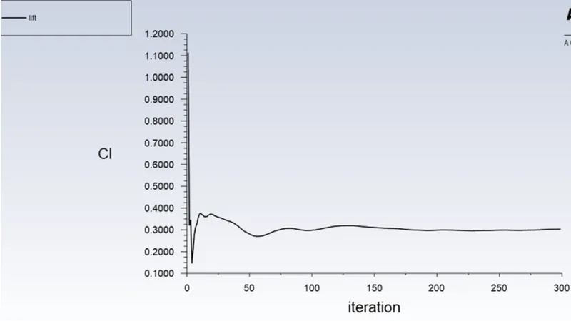
Lift co-efficient:

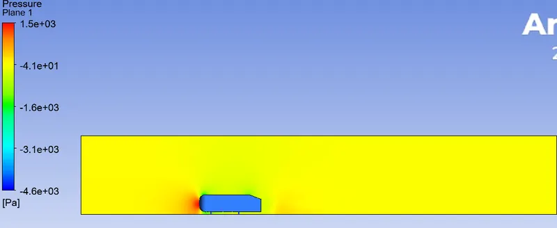
Pressure contour:

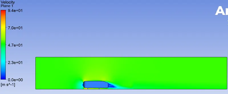
Velocity contour:

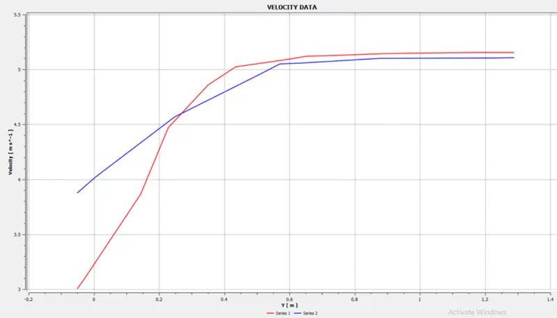
Plots:

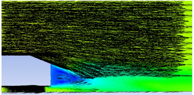
Vectors:

Conclusion:

1. The simulation of the Ahmed Body runs well and is in some agreement with experimental and empirical data on the body.
2. There are regions behind the body where wakes are formed, circling regions of low velocity which induce a considerable amount of velocity drag on the body.
3. The values of drag coefficient agree with almost all publications, although there is limited data for a slant angle of 20 degrees for the Ahmed Body.
4. The values of lift coefficient agree with some sources and disagree with others, this discrepancy is due to coarser mesh around the botton region of the ahmed body.