Project 2 - Rankine cycle Simulator

Aim: To create a Rankine Cycle Simulator using OCTAVE/MATLAB.

Objectives:

• To calculate the state points of the Rankine cycle.
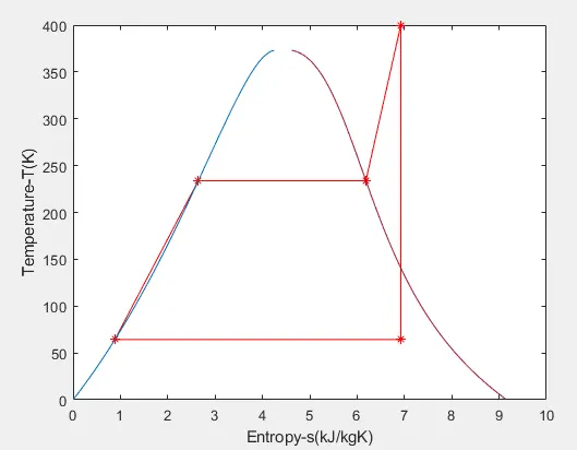
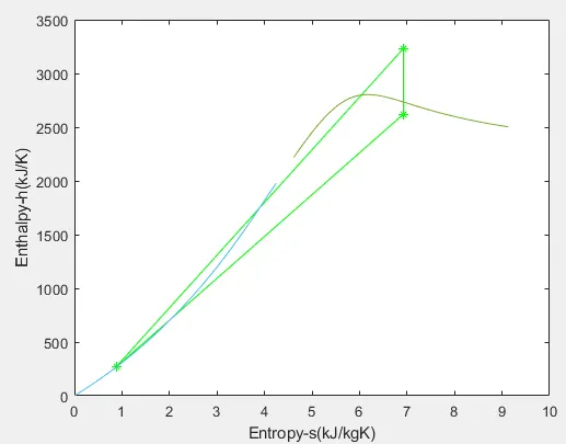
• Plot the corresponding T-s and h-s plots.

Theory:

Rankine cycle:

A Rankine cycle is an ideal cycle which governs the working of a heat engine. There are four different components which works on different processes. They are turbine, condensor, pump and boiler.

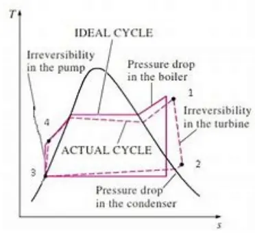
1-2: Isentropic expansion in the turbine

2-3: constant pressure heat rejection in the condensor

3-4: isentropic compression in pump

4-1: constant pressure heat addition in the boiler

Thermodynamic equations:

For isentropic expansion:

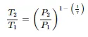
T = temperature at the state (K),

P = pressure at the state (Bar),

gamma = heat capacity ratio

For net work (W_net) and back work ratio (Bw_ratio):

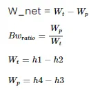
h = enthalpy at that state (kJ/kg)

W_t = turbine work (kJ/kg)

W_p = pump work (kJ/kg)

Thermal efficiency:

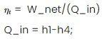
Q_in = heat added by the boiler (J)

Description of the program:

(1) The given inputs are entered.

(2) Using XSteam data and thermodynamic equation, various state variables are calculated.

(3) Net work done, back work ratio and thermal efficiency are found.

(4) T-s and h-s diagrams are plotted.

Program:

%Rankine cycle
close all
clear all
clc

disp('RANKINE CYCLE');
disp('1-2 is Isentropic Expansion in the Turbine');
disp('2-3 is Constant Pressure Heat Rejection by the Condensor');
disp('3-4 is Isentropic Expansion in the Pump');
disp('1-2 is Constant Pressure Heat Addition to the Boiler');

%Inputs
disp('INPUTS');
P1=input('Enter the Pressure at turbine inlet(bar):');
T1=input('Enter the Temperature at the Turbine inlet(degree C):');
P2=input('Enter the Pressure at the Condensor(bar):');

%Using the Xsteam functions, enthalpy and entropy at various points can be
%calculated

%Calculating enthalpy(h) and entropy(s) at point 1:
h1=XSteam('h_pT',P1,T1);
s1=XSteam('s_pT',P1,T1);

%Calculating pressure(P),enthalpy(h) and entropy(s) at point 2
%Since isentropic expansion
s2=s1;

%For isentropic expansion, (T2/T1)=(P2/P1)^(1-(1/g))
g=1.4;
power=1-(1/g);
T2=T1*((P2/P1)^power);
h2=XSteam('h_pT',P2,T2);

%Calculating pressure, enthalpy and entropy at point 2
%Since constant pressure heat removal
P3=P2;
T3=T2;
h3=XSteam('hL_T',T3);
s3=XSteam('sL_T',T3);

%Caluculating pressure, enthalpy and entropy at point 4
%Since isentropic compression
s4=s3;

%Since constant pressure proces
P4=P1;
T4=XSteam('T_ps',P4,s4);
h4=XSteam('h_pT',P4,T4);
h41=XSteam('hL_p',P4);
s41=XSteam('sL_p',P4);
h42=XSteam('hV_p',P4);
s42=XSteam('sV_p',P4);
T41=XSteam('T_hs',h41,s41);
T42=XSteam('T_hs',h42,s42);

%Calculating entropy and enthalpy at the saturation curve
Temp=linspace(0,500,600);
for i=1:length(Temp)
    sv(i)=XSteam('sV_T',Temp(i));
    sl(i)=XSteam('sL_T',Temp(i));
    
    hv(i)=XSteam('hV_T',Temp(i));
    hl(i)=XSteam('hL_T',Temp(i));
end

%Calculating the net work output (W_net)
W_t=h1-h2;
W_p=h4-h3;
W_net=W_t-W_p;

%Calculating back work ratio
Bw_ratio=W_p/W_t;

%Calculating thermal efficiency
Q_in=h1-h4;
eff_thermal=(W_net/Q_in)*100;

%Calculating sepcific steam consumption, 1J=3600 kg/s
SSC=3600/W_net;

%Displaying results in the command window
disp('Results');
P1=P1;
T1=T1;
P2=P2;
disp('At stage point 1');
n1=sprintf('P1 is %.3f bar',P1);
disp(n1);
n2=sprintf('T1 is %.3f C',T1);
disp(n2);
n3=sprintf('h1 is %.3f kJ/kg',h1);
disp(n3);
n4=sprintf('s1 is %.3f kJ/kgK',s1);
disp(n4);
disp('At stage point 2');
n11=sprintf('P2 is %.3f bar',P2);
disp(n11);
n21=sprintf('T2 is %.3f C',T2);
disp(n21);
n31=sprintf('h1 is %.3f kJ/kg',h2);
disp(n31);
n41=sprintf('s2 is %.3f kJ/kgK',s2);
disp(n41);
disp('At stage point 3');
n12=sprintf('P3 is %.3f bar',P3);
disp(n12);
n22=sprintf('T3 is %.3f C',T3);
disp(n22);
n32=sprintf('h3 is %.3f kJ/kg',h3);
disp(n32);
n42=sprintf('s3 is %.3f kJ/kgK',s3);
disp(n42);
disp('At stage point 4');
n13=sprintf('P4 is %.3f bar',P4);
disp(n13);
n23=sprintf('T4 is %.3f C',T4);
disp(n23);
n33=sprintf('h4 is %.3f kJ/kg',h4);
disp(n33);
n43=sprintf('s4 is %.3f kJ/kgK',s4);
disp(n43);
n14=sprintf('W_t is %.3f kJ/kg',W_t);
disp(n14);
n15=sprintf('W_p is %.3f kJ/kg',W_p);
disp(n15);
n16=sprintf('W_net is %.3f kJ/kg',W_net);
disp(n16);
n17=sprintf('Eff_Thermal is %.2f Percent',eff_thermal);
disp(n17);
n18=sprintf('SSC is %.2f kg/kWh',SSC);
disp(n18);


figure(1)
plot([s1 s2],[T1 T2],[s2 s3],[T2 T3],[s3 s4],[T3 T4],[s4 s41],[T4 T41],[s41 s42],[T41 T42],[s42 s1],[T42 T1],'marker','*','color','r')
hold on
plot(sv,Temp)
plot(sl,Temp)
xlabel('Entropy-s(kJ/kgK)');
ylabel('Temperature-T(K)');

figure(2)
plot([s1 s2],[h1 h2],[s2 s3],[h2 h3],[s3 s4],[h3 h4],[s4 s1],[h4 h1],'marker','*','color','g')
hold on
plot(sv,hv)
plot(sl,hl)
xlabel('Entropy-s(kJ/kgK)');
ylabel('Enthalpy-h(kJ/K)');

Output:

T-S diagram:

H-S diagram:

Results and conclusion:

• Performance of the heat engine is calculated and the observations are followed:

(1) Net work = 608.093 kJ/kg

(2) Thermal efficiency = 20.55%

(3) Back work ratio = 0.004%

The T-S and H-S graphs are plotted.