Week 4.1 - Genetic Algorithm

Aim:

• Write a code in MATLAB to optimise the stalagmite function and find the global maxima of the function.

Objective:

• To study about genetic algorithm and stalagmite function.
• To write a code in Matlab to optimize the stalagmite function and to find the global maxima of the function.
• To plot graphs based on the study.

Theory:

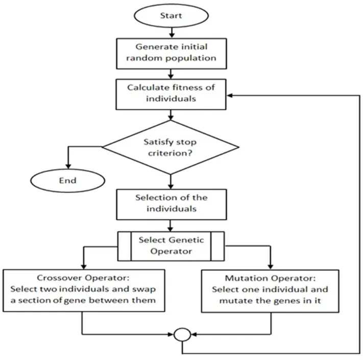
Genetic algorithm works on the principle of natural selection, where fittest individuals are selected for reproduction inorder to produce offspring of the next generation. It is method used for solving both constrained and unconstrained optimization problems that is based on natural selection. The basic steps involved in creating a genetic algorithm is as follows:

• The algorithm creates a random initial population in the beginning.
• To create a new population, the algorithm scores each member of the current population by computing its fitness value and coverts them to a more usable range of values.
• Based on these new values, algorithm selects members, called parents.
• Algorithm then produces children from these parents.
• In this way, algorithm replaces the current population with children to form the next generation.
• The algorithm stops when it reaches any one of the specified factors, such as time limit, fitness limit, generations, function tolerance etc.

The flowchart for genetic algorithm is as follows:

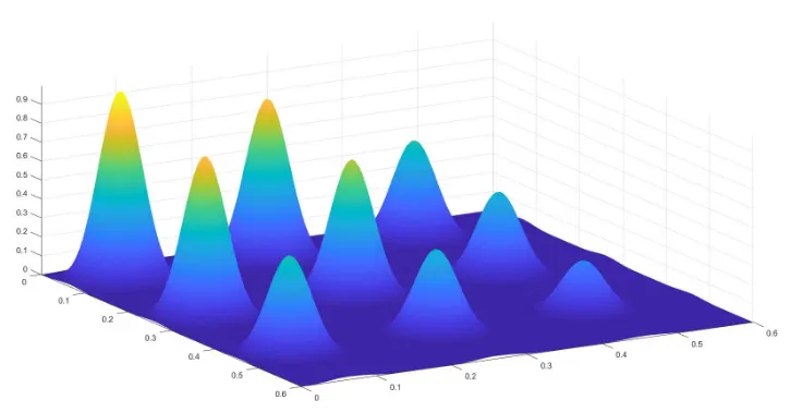
Stalagmite function: It is a mathematical model which is used to find local maxima and minima. It has lots of local maxima and minima and one global maxima or minima.

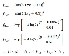
The stalagmite function is given as:

Matlab program:

Function for stalagmite function:

function[f]= stalagmite(input_vector)
  fx=(sin(5.1*pi*input_vector(1)+0.5))^6;
  fy=(sin(5.1*pi*input_vector(2)+0.5))^6;

  fxx=exp((-4*log(2)*(((input_vector(1)-0.0667)^2)/0.64)));
  fyy=exp(-4*log(2)*(((input_vector(2)-0.0667)^2)/0.64));
  
  f=-(fx*fy*fxx*fyy);
end

Negative sign in the function will invert the stalagmite plot which gives the function maxima.

Code for Genetic Algorithm:

close all
clear all
clc

num_cases=150;

x=linspace(0,0.6,150);
y=linspace(0,0.6,150);
[xx yy]=meshgrid(x,y);



for i=1:length(xx)
  for j=1:length(yy)
    input_vector(1)=xx(i,j);
    input_vector(2)=yy(i,j);
    f(i,j)= stalagmite(input_vector);
  end
end

%1st case
tic
for i=1:num_cases
 [inputs,fopt(i)]= ga(@stalagmite,2);
  xopt(i)=inputs(1);
  yopt(i)=inputs(2);
end
fopt=-fopt;
time_study1=toc



figure(1)
subplot(2,1,1)
hold on
surfc(x,y,-f)
shading interp
plot3(xopt,yopt,fopt,'marker','o','markersize',5,'markerfacecolor','r')
title('Unbound inputs')
%figure(2)
subplot(2,1,2)
plot(fopt)
xlabel('Iteration')
ylabel('Function minimum')





%study2



tic
for i=1:num_cases
 [inputs2,fopt2(i)]= ga(@stalagmite,2,[],[],[],[],[0,0],[1,1]);
  xopt2(i)=inputs2(1);
  yopt2(i)=inputs2(2);
end
fopt2=fopt2;
time_study2=toc

figure(2)
subplot(2,1,1)
hold on
surfc(x,y,f)
shading interp
plot3(xopt2,yopt2,fopt2,'marker','o','markersize',5,'markerfacecolor','r')
title('Bounded inputs')
%figure(2)
subplot(2,1,2)
plot(fopt2)
xlabel('Iteration')
ylabel('Function minimum')




%Case_study 3: MAximising the population size to optimise the result


options= optimoptions ('ga');
options=optimoptions(options,'PopulationSize',500);

tic
for i=1:num_cases
  [inputs3, fopt3(i)]=ga(@stalagmite,2,[],[],[],[],[0,0],[1,1],[],[],options);
  xopt3(i)=inputs3(1);
  yopt3(i)=inputs3(2);
end
figure(3)
subplot(2,1,1)
hold on
surfc(x,y,-f)
shading interp
plot3(xopt3,yopt3,-fopt3,'marker','o','markersize',5,'markerfacecolor','r')
title('Bounded inputs with optioptims function')
subplot(2,1,2)
plot(-fopt3)
xlabel('Iteration')
ylabel('Function minimum')

time_study3=toc
rng('default');

Results:

Study 1 : Statistical behaviour

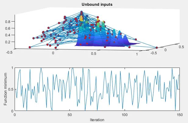
From this plot, it is observed that the random sampling of the genetic algorithm generates a new maximum value for the function every time the code is run.

Study 2: Statistical behaviour with upper and lower bounds

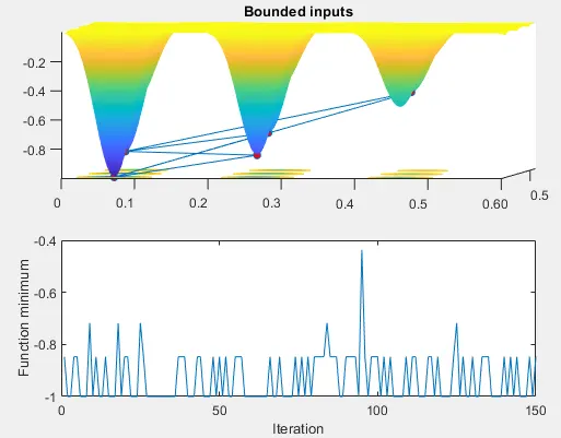
This shows the convergence of x and y values.

Study 3: Statistical behaviour with increasing number of iterations

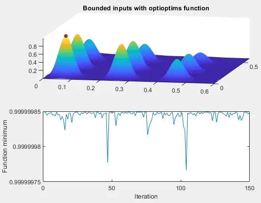
Here, there is only one red dot, which is the required global maxima.

Conclusion:

The require glovbal maxima and local maxima and minima is found out using genetic algorithm method, including stalagmite function.