Week 3 - External flow simulation over an Ahmed body.
im:- Ahmed body analysis.
Objective:-
Run the simulation for the velocity of 25 m/sec with the default air properties in fluent.
Q1. Describe Ahmed's body and its importance.
Q2. Explain the reason for the negative pressure in the wake region.
Q3. Explain the significance of the point of separation.
Expected Results:
- Velocity and pressure contours.
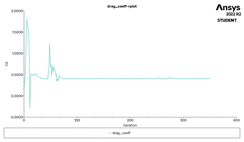
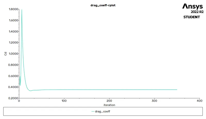
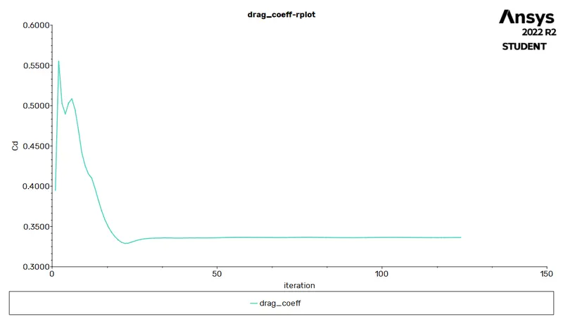
- The drag coefficient plot for a refined case. (For velocity of 25m/sec, the drag coefficient should be around 0.33).
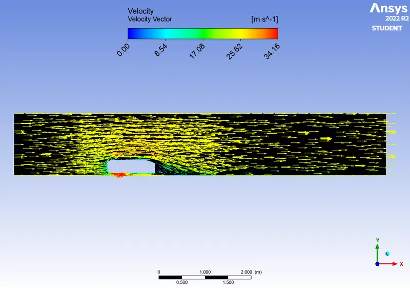
- The vector plot clearly showing the wake region.
- Perform the grid independency test and provide the values of drag and lift with each case
Theory:- Ahmed Body
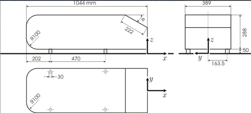
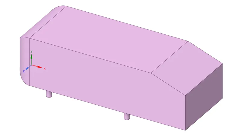
The Ahmed body is a generic car body (a simplified vehicle model). The airflow around the Ahmed body captures the essential flow features around an automobile and was first defined and characterized in the experimental work of Ahmed. Although it has a very simple shape, Ahmed body allows us to capture characteristic features that are relevant to bodies in the automobile industry.
This model is also used to describe the turbulent flow field around a car-like geometry. Once the numerical model in validated, it is used to design new models of the car.
dimesion of ahmed body.
Importance Of ahmed body
1. We can simulate the fundamental physics on the ahmed body, which can be validate and used to design new cars.
2. We can analys the flow sepration and weak reasong formation.
3. We can analyse the drag lift velocity and other important aspects.
4. We can analyse the effect of slant angle over the car bodies.
Reason for the negative pressure in the wake region
Negative Pressure in the wake region is created because of velocity difference and sudden change in geometry
Significance of Point of Sepration
Point of sepration have a great significance in understanding the fluid flow over a car body. The point of speration depend upon the geometry of the system body and the flow properties. generation of weak region is depend on the point of sepration

Y+ model
The behaviour of the flow near the wall is a complicated phenomena and to distingish the different region near the wall the concept of wall has been formulated. This is the dimesnion less qunatity, and the distance from the wall measured in terrm of visous length
To resolve the effect near the wall i.e. inthe viscous sublayer then the size of the mesh should be small and dense enough near the wall so that almost all the effect can be captured
When any viscous flow flows over a surface, a region of slow-moving flow called boudary layer develops.
inside the boundary layer, there is a strong velocity gradient and u varies nonlinearly
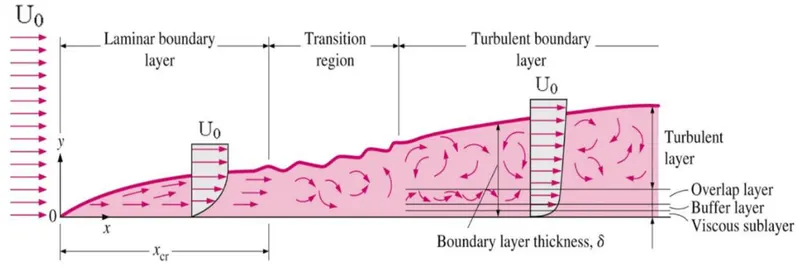
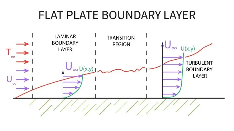
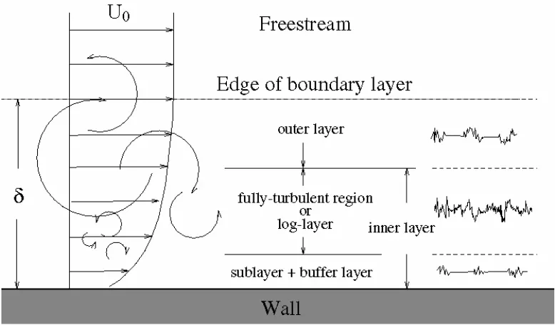
it is very important to distinguish between different layers to model the boundary physics correctly
For CFD SImulation we can compute the frist layer thickness values using online calculator
to calculate frist layer thickness we must have
1. free stream velocity
2. denisty of the fluid
3. dynamic viscosity
4. refrence length
5. refrence value for y+
Some refrence values for y+ are
for viscous layer .1 to 5
for buffer layer 5 to 30
for inertial sublayer 30 to 100
defect layer 1000 to 10000
for some models
for k-omega 1 to 10
for k-epsilon 30 to 100
for k-Omega sst 0 to 5
CFD:-Computational fluid dynamics or CFD is the analysis of systems involving fluid flow, heat transfer and associated phenomena such as chemical reactions by means of computer-based simulation.
Practical application in current scenario
- aerodynamics of aircraft and vehicles: lift and drag
• hydrodynamics of ships
• power plant: combustion in internal combustion engines and gas
turbines
• turbomachinery: flows inside rotating passages, diffusers etc.
• electrical and electronic engineering: cooling of equipment including
microcircuits
• chemical process engineering: mixing and separation, polymer moulding
• external and internal environment of buildings: wind loading and
heating/ventilation
• marine engineering: loads on off-shore structures
• environmental engineering: distribution of pollutants and effluents
• hydrology and oceanography: flows in rivers, estuaries, oceans
• meteorology: weather prediction
• biomedical engineering: blood flows through arteries and veins
CFD Work Flow:- CFD codes are structured around the numerical algorithms that can tackle fluid flow problems. In order to provide easy access to their solving power all commercial CFD packages include sophisticated user interfaces to input problem parameters and to examine the results
Its threee step process
(i) a pre-processor
involves defination of geometry, grid generation, selection of phenomenon that need to model
(ii) a solver
intergration of governing equation, discretisation and solution
(iii) a post-processor
ploting of contour, graphs and making movies.
In solving fluid flow problems we need to be aware that the underlyingphysics is complex and the results generated by a CFD code are at best asgood as the physics (and chemistry) embedded in it and at worst as good asits operator with CFD
Solving and Modeling Approch:-
There are no way present to understand and analyse the effeciveness of the mixiing tee model.
1. analytical approch
2. simulation approch
3. experimental approch
using analytical approch and experimental approch is time consuming and high cost senario. this could be eliminated by using simulation approch in which we can analyse the system with the actual codition we are intrested in.
To do this we are using ansys fluent solver
we are using fluid flow analysis using Fluent solver because we are interested in the total effectiveness of the fluid in the mechnical tee model, here we are using two different models to analyse the effectiveness of the mixing of fluid.
Approch we are using.
1. We need to open Ansys workbench
2. Choose the Appropiate Solver
3. Assign Appropiate name
4. Choose geometry and select new spaceclaim model.
5. Load the appropiate file
6. Implement the geometrical operation
7. Apply the mesh and provide name selection
8. Choose setup, select the appropiate model
9. Initalisation and running the simulation
10. Result making i.e. countour plots graphs
Preprocessing and Solver setting
1. Opening Ansys workbench
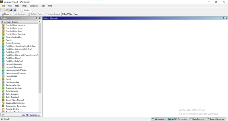
2. Choose the Appropiate Solver
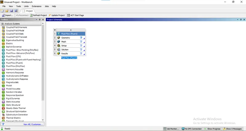
3. Assign Appropiate name
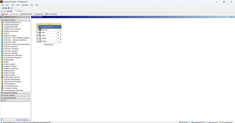
4. Choose geometry do to geometrical operation
choose the geometry>right click and choose spaceclaim>choose the file
change the units.
file>space claim option>units> change mm to meter
use measure tool so as to calculate the hydraulic diameter
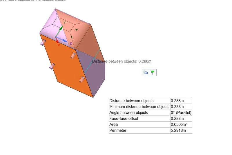
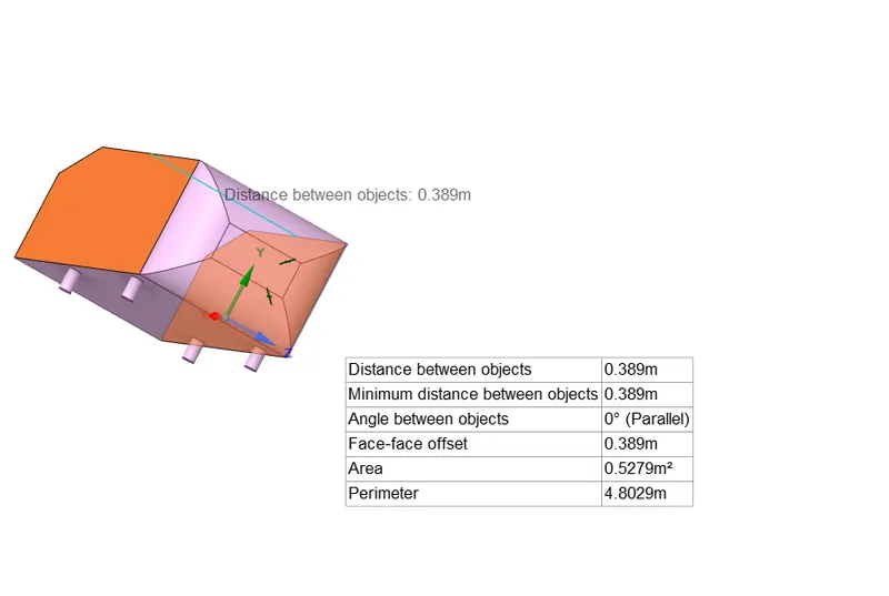
measure distance are width is .389m and height is .288m
in order to prepare the enclosure
go to preapre>enclosure>disable the symmetry(because we have different length of enclosure in front and back side)
create a enclosure with
1. frist enclosure
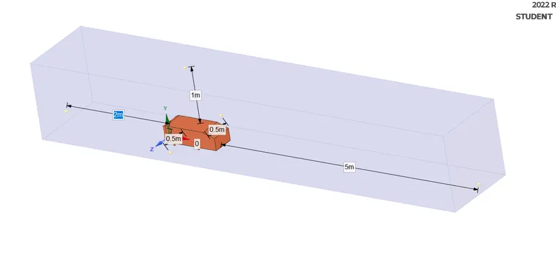
Here we create two enclosure just to limit the no. of elements.
2. Second enclosure
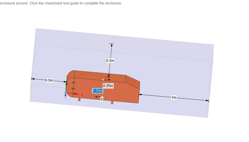
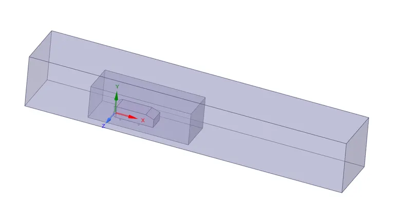
now we need to create planes
design>plane>select origin point>it create 3 planes
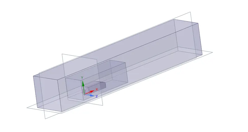
to see cut section view go to design>cut section >select the plane with repective we want cut sectional view
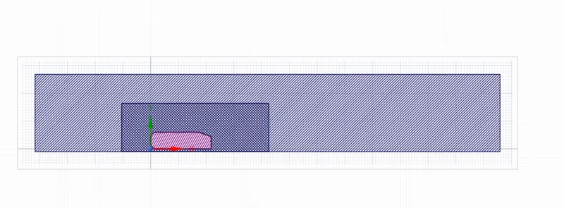
after observing cut sectional view we find that there are interference surfaces. to eliminate this we use interference
go to prepare>interference>click on right symbol
it will delete the interfernce/overlapping surfaces.
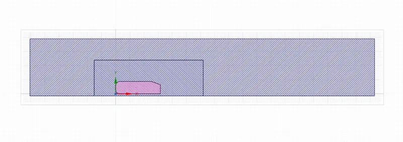
Now we need to use share the topology, just to ensure that connected body have shared faces
go to workbench>share>click ok
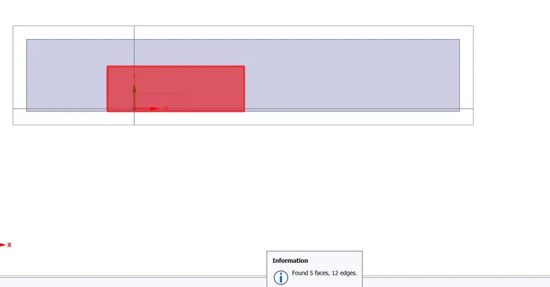
click on green right.
We completed the geometry part
Meshing:-
now we open mesh window
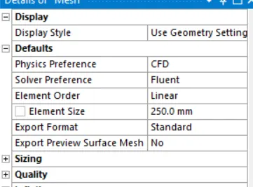
1. click on the mesh and choose base element length as 250mm i.e. click on generate mesh
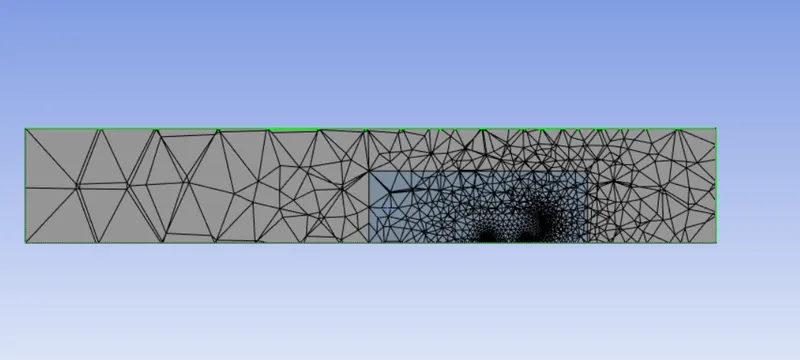
choose base mesh as 250mm
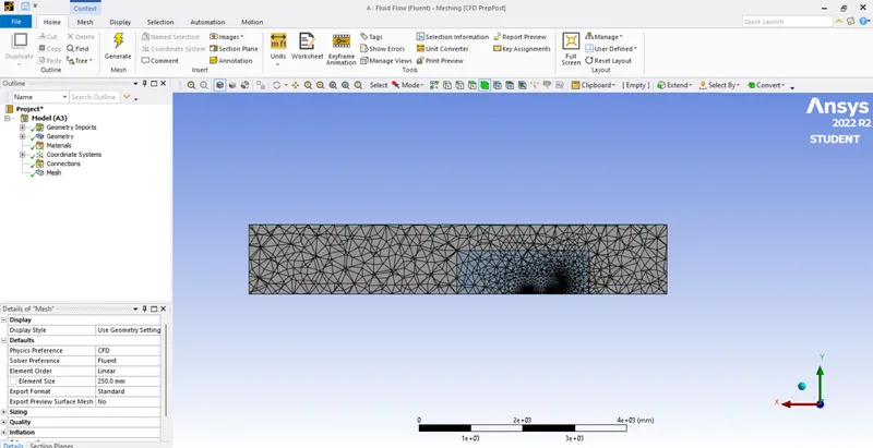
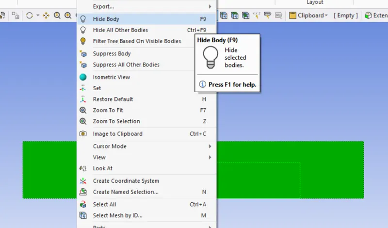
No hide the upper enclosure by selecting body>right click and hide
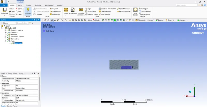
now we use insert sizing method to provide mesh length of 100mm to inner enlosure.
mesh>insert>sizing>select the body>select apply>provide mesh length as 100mm.
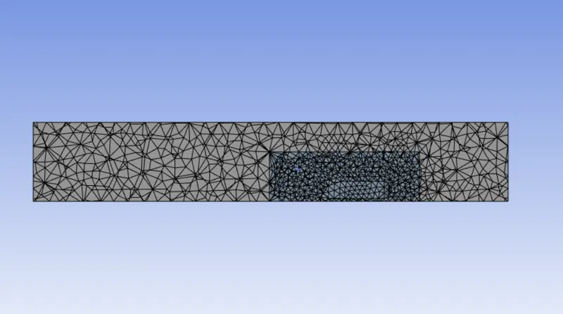
We observe that the cylindrical holes at the buttom are not in perfect shape
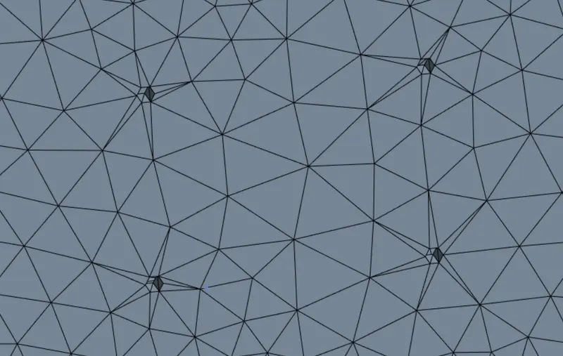
to correct them we need to use sizing method.
mesh>insert>sizing>select the body(selection will be in blue color)>select apply>provide mesh length as 5 mm
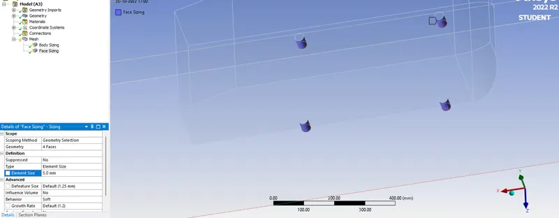
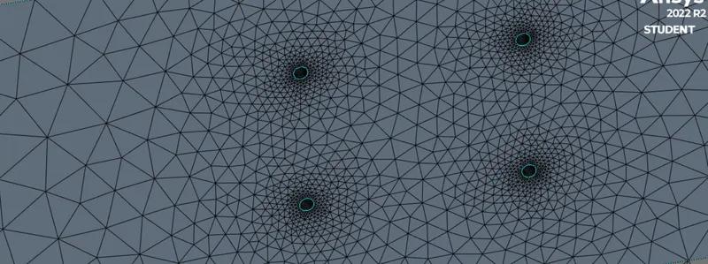
Now provide the name selection
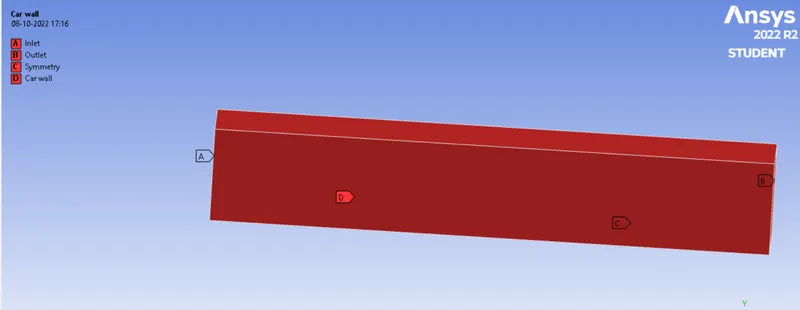
Now we provide the inflation layers
mesh>insert>inflation>select the body(selection will be in blue color)>select apply>provide mesh length as .4 mm
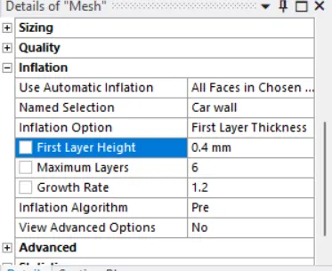
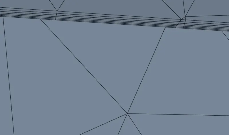
Now we completed with meshing.
Setup:-
Settings
| Solver | Steady State |
| Energy Equation | Off |
| Model | K-epsilon |
| Inlet | Inlet Velocity |
| Outlet | Pressure Outlet |
| Material_(Fluid) | Air |
| Cell Zone Condition | Air |
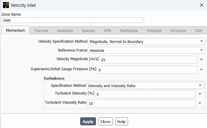
| Boundary Condition | Velocity Input 25m/s |
Refrence Value
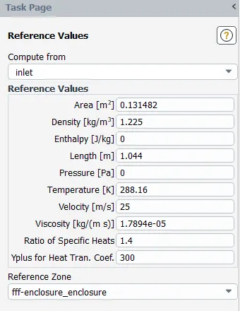
Setting Boundary Condition
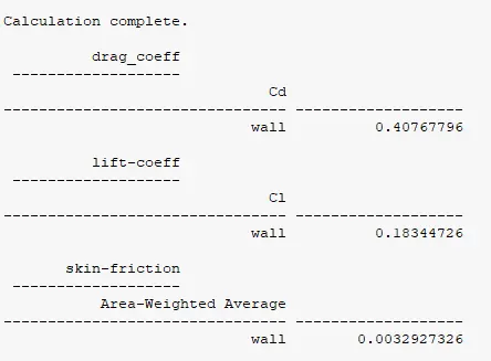
Results Needed
1. Drag Coefficient graph
2. Lift Coefficient graph
3. Skin friction coefficient
4. Residual Plot
5. Velocity Contour
6. Pressure Contour
Mesh length
base mesh 250mm
ineer enclosure 100mm
for sylindrical pillar 5mm
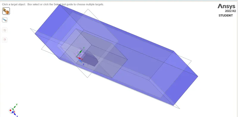
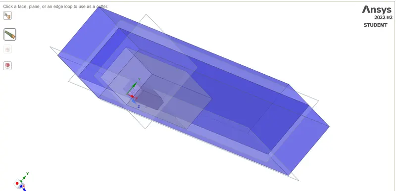
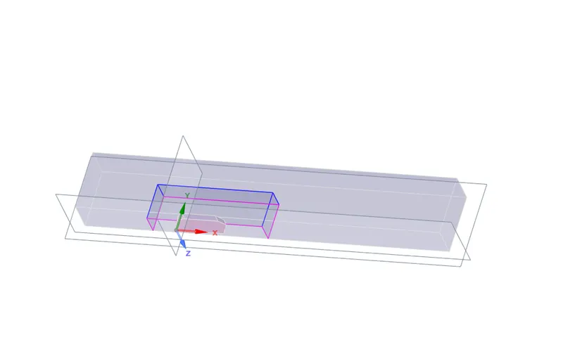
Split Body
Now we perform the study using spilt body, jsut to reduce the computaional time As it is a symmetry body we can spilt the body. and perform the analysis
Rest procedure is same in geometry for creating enclosure and all. Before performing interference and share topology we need to use slpit body command
Go to design >split body> select the target>click on cutter>select the plane>select regions to remove
base mesh 100mm
ineer enclosure 50mm
for sylindrical pillar 3mm
base mesh 50mm
ineer enclosure 40mm
for sylindrical pillar 3mm
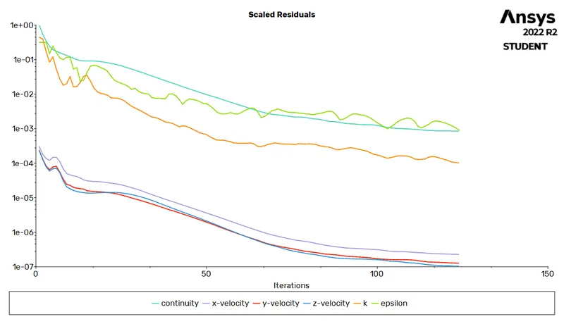
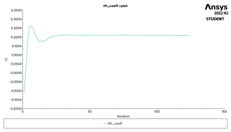
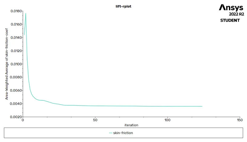
solution became conversed at 124 iteration.
Results
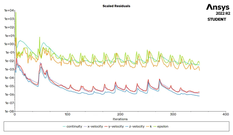
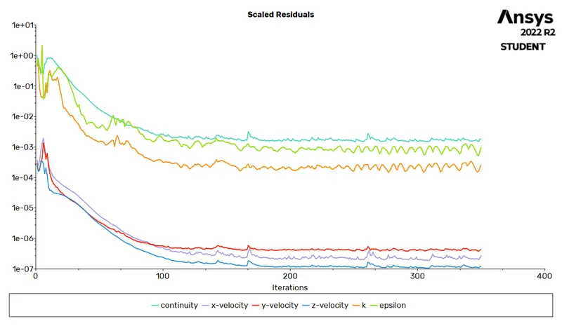
1. Residuals
|
Mesh length 250mm Inner enclosure 100mm Cylinder 5mm |
Mesh length 100mm Inner enclosure 50mm Cylinder 3mm |
Mesh length 50mm Inner enclosure 40mm Cylinder 3mm |
 |
 |
 |
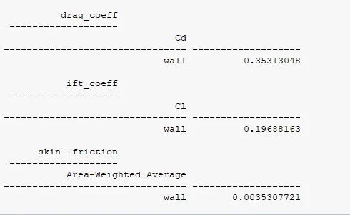
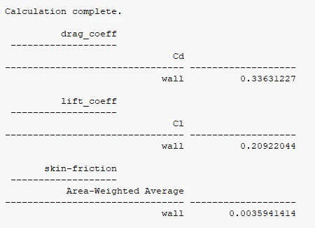
2. Drag Coefficient
|
Mesh length 250mm Inner enclosure 100mm Cylinder 5mm |
Mesh length 100mm Inner enclosure 50mm Cylinder 3mm |
Mesh length 50mm Inner enclosure 40mm Cylinder 3mm |
 |
 |
 |
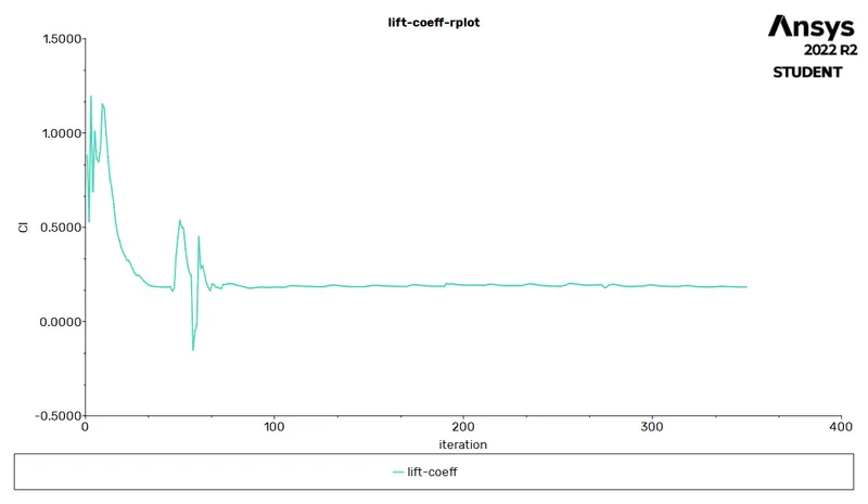
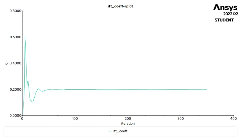
3. Lift Coefficient
|
Mesh length 250mm Inner enclosure 100mm Cylinder 5mm |
Mesh length 100mm Inner enclosure 50mm Cylinder 3mm |
Mesh length 50mm Inner enclosure 40mm Cylinder 3mm |
 |
 |
 |
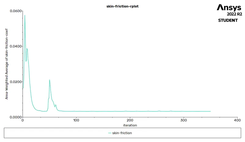
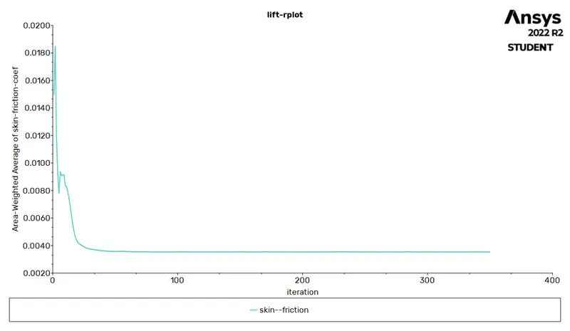
4. Skin friction
|
Mesh length 250mm Inner enclosure 100mm Cylinder 5mm |
Mesh length 100mm Inner enclosure 50mm Cylinder 3mm |
Mesh length 50mm Inner enclosure 40mm Cylinder 3mm |
 |
 |
 |
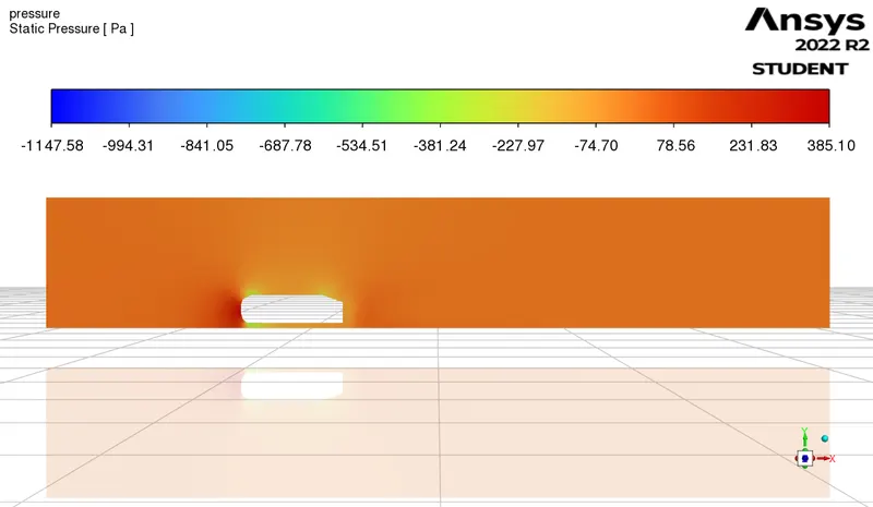
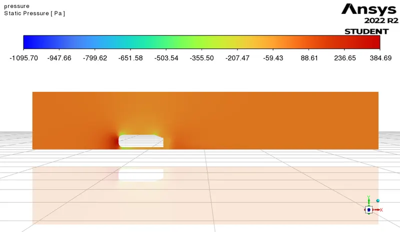
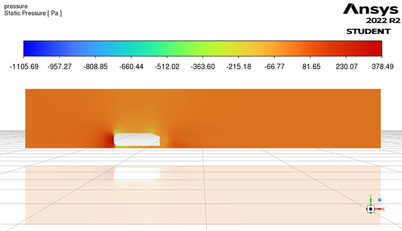
5. Presure Contour
|
Mesh length 250mm Inner enclosure 100mm Cylinder 5mm |
Mesh length 100mm Inner enclosure 50mm Cylinder 3mm |
Mesh length 50mm Inner enclosure 40mm Cylinder 3mm |
 |
 |
 |
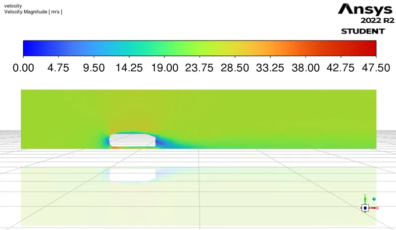
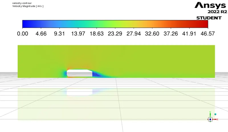
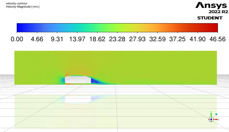
6. Velocity Contour
|
Mesh length 250mm Inner enclosure 100mm Cylinder 5mm |
Mesh length 100mm Inner enclosure 50mm Cylinder 3mm |
Mesh length 50mm Inner enclosure 40mm Cylinder 3mm |
 |
 |
 |
7. Coefficient
|
Mesh length 250mm Inner enclosure 100mm Cylinder 5mm |
Mesh length 100mm Inner enclosure 50mm Cylinder 3mm |
Mesh length 50mm Inner enclosure 40mm Cylinder 3mm |
|
|
|
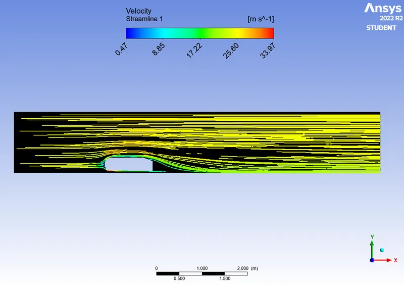
| Velocity vector | Streamline |
 |
 |
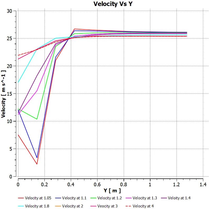
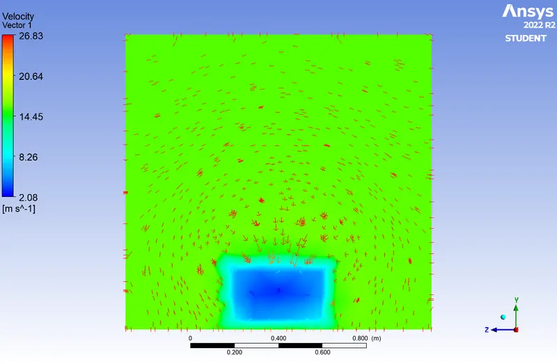
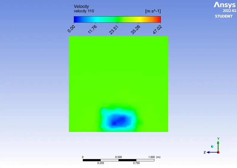
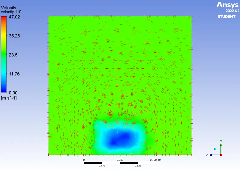
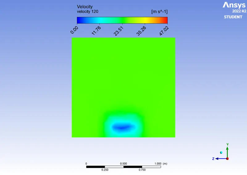
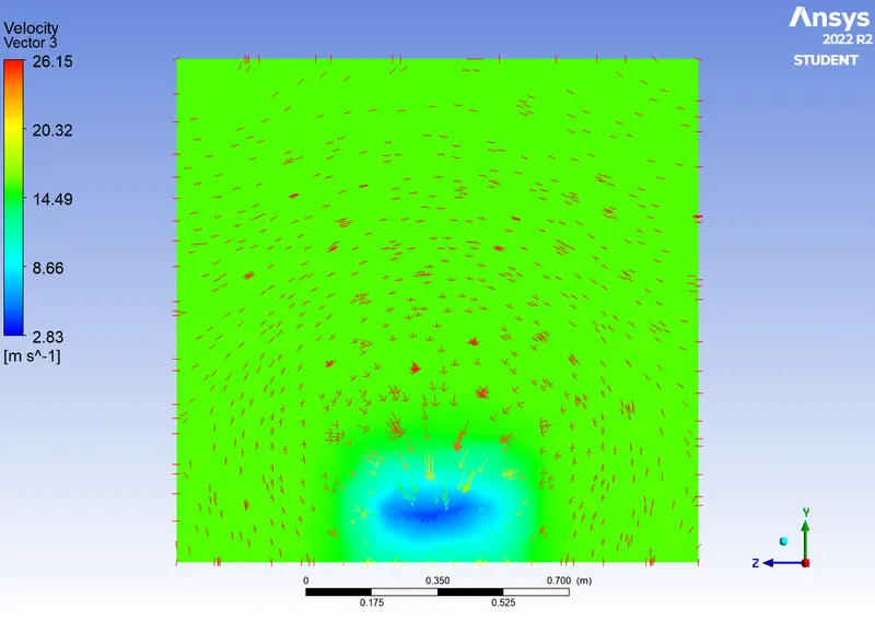
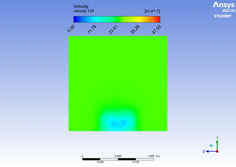
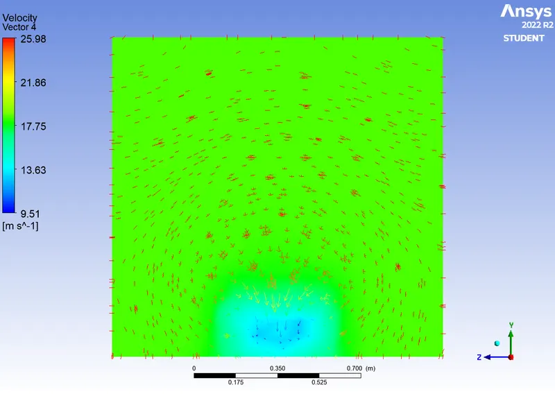
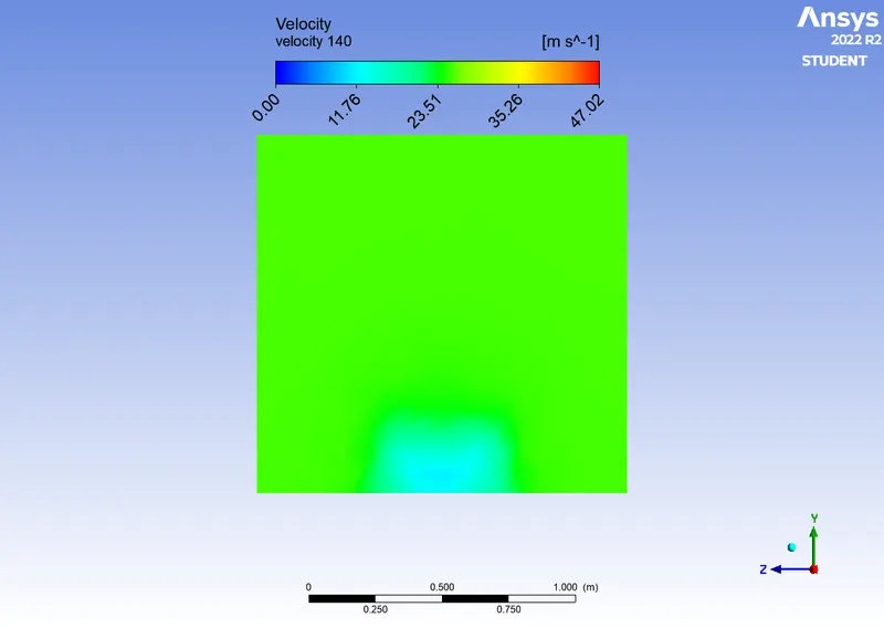
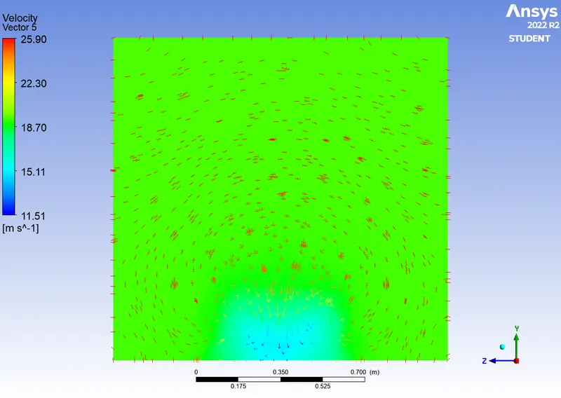
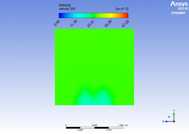
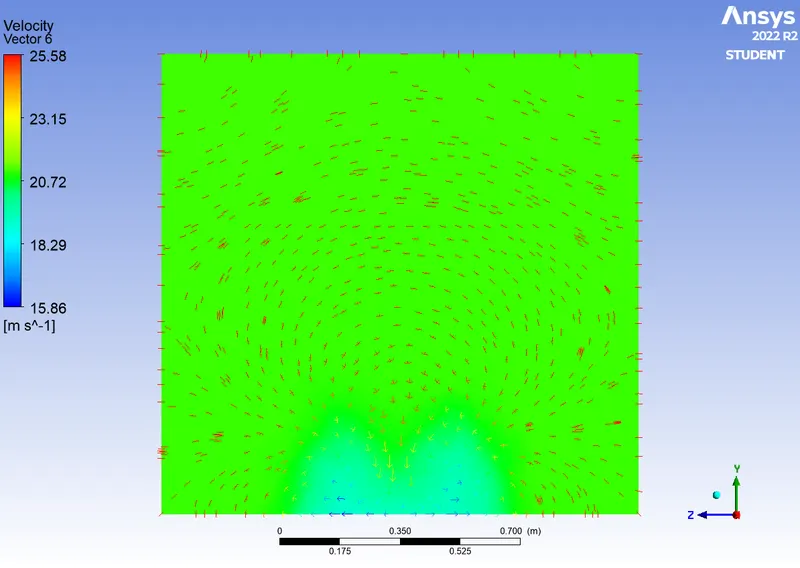
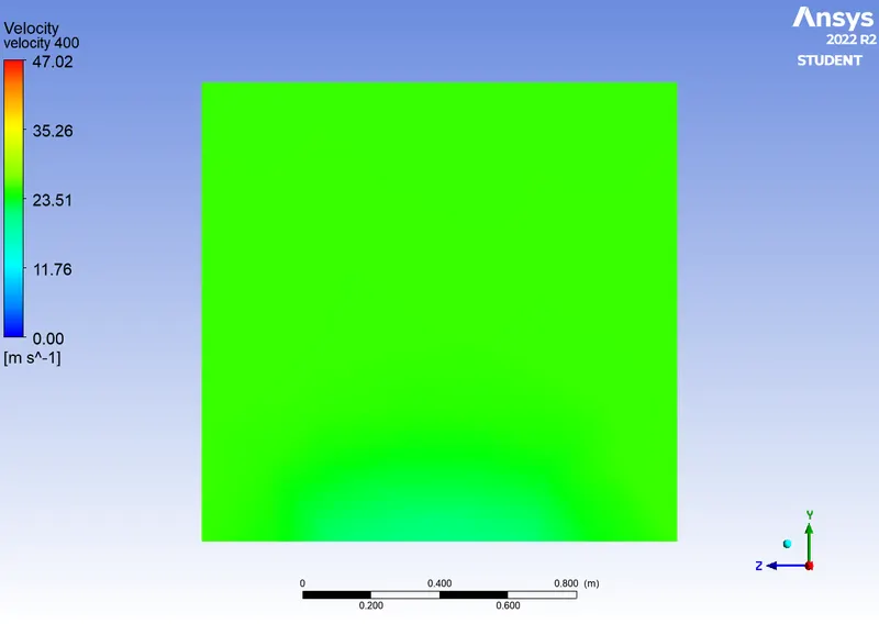
Velocity chart at different location
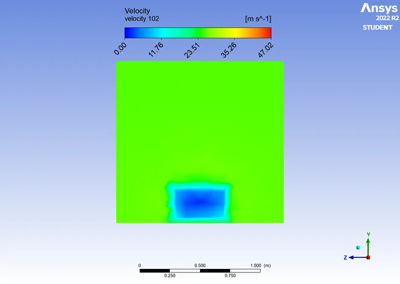
| Velocity contour | Velocity Vector |
 |
 |
 |
 |
 |
 |
 |
 |
 |
 |
 |
 |
 |
 |
Inferences:-
1. intensity of velocity iincreases as we move in right direction
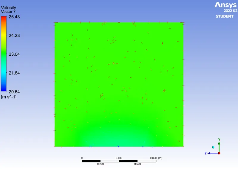
2. Weak region last upto 1.04 to 1.47m
3. velocity vs y, velocity increases as we move in +y direction
4. high pressure generated at front side due to direct connect and large forntal area
5. velocity is low at weak region
6. as we fine the mesh size we get accurate results. and chance of getting conversed solution increases.
7. weak region i.e. negative pressure region are formed behind the ahmed body
8. as its a symmetric body we can spilit the body into two halfs and we can reduce the overall calculation time.
Reference Research papers: