Week 3 - External flow simulation over an Ahmed body.

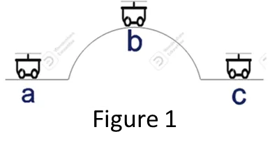
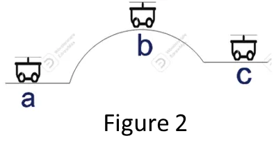
Let us imagine a roller coaster(R) having a specific path as represented in figure 1. Now consider R being in movement and moving at a considerably large velocity. Thus we can say that at point a, the roller coaster has total energy equal to its Kinetic energy. While it makes up to point b, the kinetic energy is completely converted into potential energy stored at that point in R. After that with respect to no energy loss it reaches point c regaining its kinetic energy. But practically there are a lot of energy losses that are to be considered like friction, heat, aerodynamic drag, etc., thus when we revisit the pathline of R, it must take a new path meeting point c in figure 2 considering all the losses. The same is the case when we deal with the fluid flow over the bodies wherein the resistance is created due to the wall shear force based on the nature of the flow. Now let us see the flow separation and the formation of the wake region behind the object in detail.

FLOW SEPARATION:

Generally, the boundary layer formation occurs when the viscous fluid flows over any solids which are either stationary or moving. When we take the fluid flow over a flat plate, it subjects to a favorable pressure gradient(Negative), that is a decrease in pressure along the length and an increase in velocity along the length(Positive velocity gradient), which makes the fluid flow and develop the boundary layer without any disturbance. However, this condition persists only till the starting of the adverse pressure gradient region wherein, from that point onwards the pressure gradient becomes positive and the velocity gradient becomes negative. Now the flow might have lost the ability to overcome the locally increased pressure and starts to split apart from the surface. This phenomenon is called Flow Separation and the point at which the flow separates is called the Point of Separation(POS) where the wall shear stress is zero. Beyond the POS, there will be the starting of reversed flow due to the negative velocity gradient. This makes the newly created reversed flow lines attach themselves to the positive direction flow lines, thus causing a rotational effect and creating vortices. These vortices must mostly be avoided since they cause unwanted vibrations and instabilities due to the match of natural frequencies of the object. Thus making a streamlined body is very important to avoid these vortex shedding.

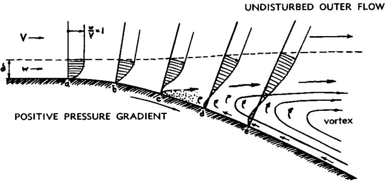
In figure 3, point c represents the Point of Separation(POS) and, beyond point c we witness the formation of negative velocity profiles which pave the way for vortex generation.

The flow separation happens at different points for a body based on the type of flow, basically, Laminar or Turbulent. For the laminar flow, the flow separation happens quickly resulting in minimal shear drag and a large pressure drag which forms a wake region(low pressure) behind the body, while for the turbulent flow, the flow separation is delayed causing minimal pressure drag but a slight increase in shear drag since the velocity profile is thicker for turbulent flow in comparison with laminar flow.

AHMED BODY AND ITS IMPORTANCE:

Firstly why do we need to study the flow characteristics of any automobile? This is because we can analyze the Total Drag formed by the shape of the vehicle which creates a negative impact on the performance of the car. Thus we will remodel the shape of the vehicle such that the total drag is reduced. In any automobile vehicle, the rear part of it contributes mainly to the development of the wake region(negative pressure). Thus in order to simplify the analysis and reduce the solution time and get an overall idea of the value of drag force, we use a generic model called Ahmed Body created by S.R. Ahmed in which we can set the rear slant angle as per our requirement. The Ahmed body is a generic car body which is a simplified car model which doesn't exactly duplicate the shape of the vehicle but helps us capture the flow characteristics over it which is very similar to that of the flow over general automotive vehicles.

STUDY:

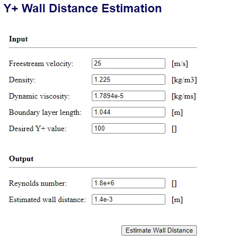
The flow over the Ahmed body can more precisely be calculated only through the consideration of the Y+ value through which the first cell height can be derived. The boundary layer length was taken as 1.044m, which is the length across the Ahmed body in the direction in which flow is simulated. The Y+ value for turbulent flow condition(Re=17e5) was considered to be 100 from the U+ vs Y+ graph. Thus from the formulae or the online resources, the first cell height was calculated to be 1.4mm.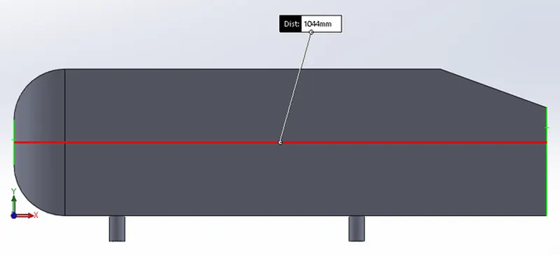

SETUP:

Geometry:

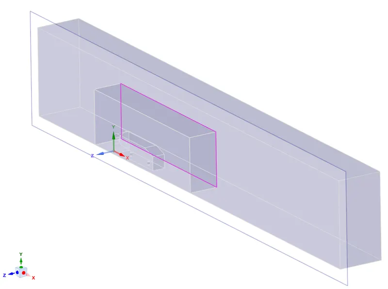
Firstly, the Ahmed body was covered with 2 enclosures with the shared topology enabled, such that the enclosures share the data effectively between the perfectly connected meshes, and then, in order to reduce the simulation time we bilaterally divided the Ahmed body along with enclosures using the split body tool.

Meshing:

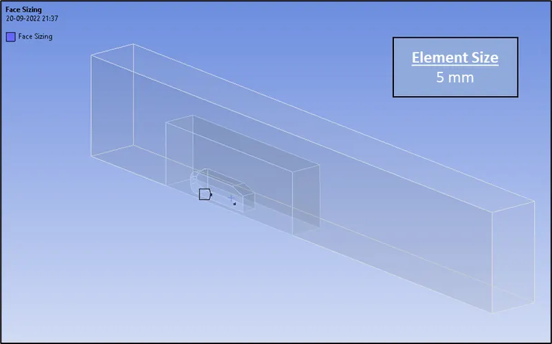
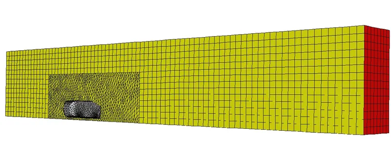
In order to prove the grid independency test, the 2 meshed structures were created, one is basic and another is refined. Both the mesh structures have a common mesh element size of 100mm for the outer enclosure and 5mm for the supporting structure. The inner enclosure had different mesh sizes that are, for basic mesh: 50mm, and refined mesh: 25mm.

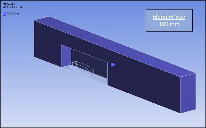
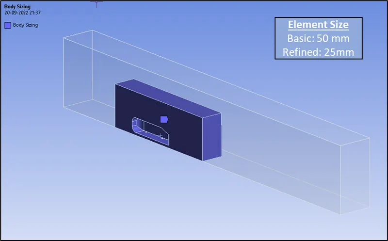
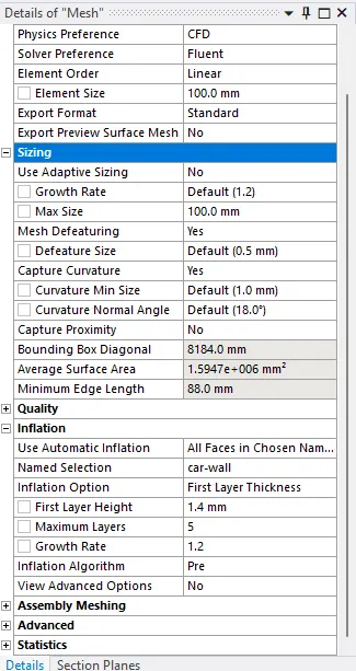
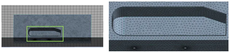
The inflation layers were added to the wall of the Ahmed body in order to capture the wall boundary layer separation effectively. The value of first layer thickness of 1.4mm which was calculated from the Y+ value seen before is made used here. The maximum number of inflation layers is 5, and 1.2 as the growth rate.

Fluent Simulation:

Basic Mesh Body(Cell count:93171):

Viscous Model: K-Omega:

Velocity & Vector Field:

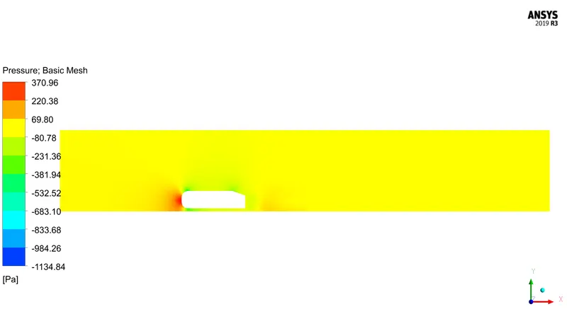
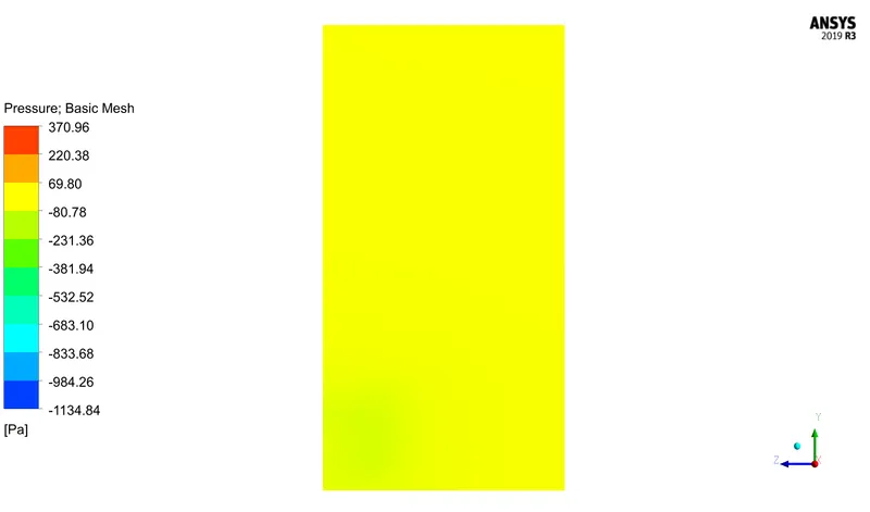
Pressure Field:

Inference from Contour Plots:

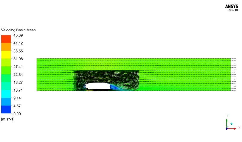
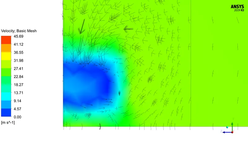
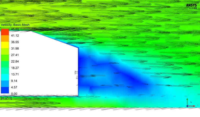
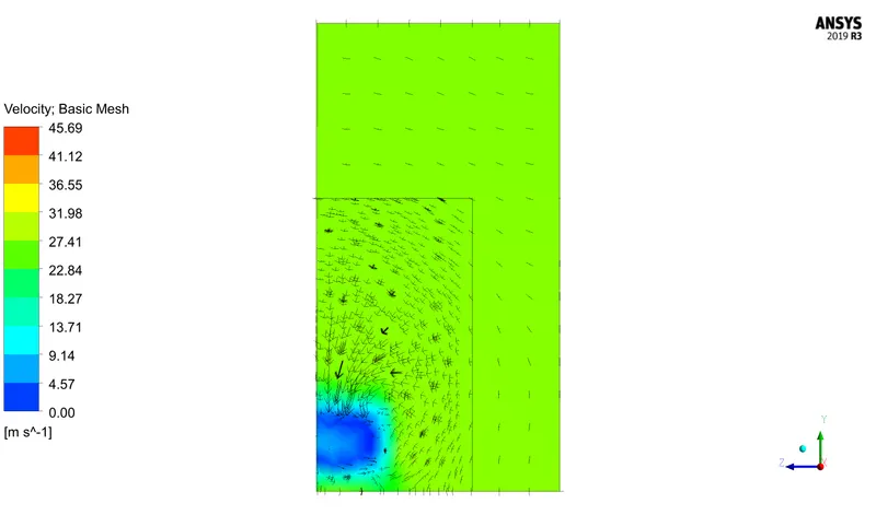
The velocity value behind the Ahmed body drops to around 12m/s to no flow condition. In the velocity vector field, we can clearly notice the boundary separation captured by the added inflation layers, and the air surrounding the Ahmed body in high pressure is being sucked into the vacuum region.

The Pressure contour says the maximum pressure is on the front of the Ahmed body where the impact due to air is more with a value of around 360Pa. The wake region behind Ahmed body has a negative pressure(around -80Pa) which is clearly visible in the cross-section contour plane in the wake region.

Results:

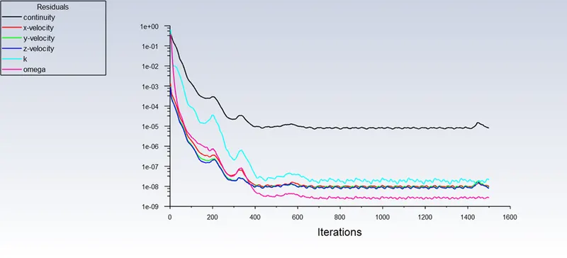
Residual Plot:

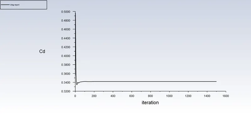
Drag Coefficient Plot:

Lift Coefficient plot:

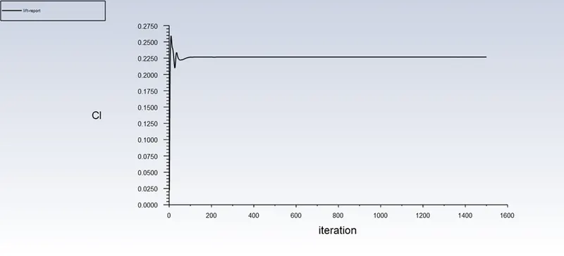
Inference from Results:

The Residual plot indicates that the simulation has come to an end and the solution has converged. And the coefficient of drag value of 0.34 was recorded. The lift coefficient value was around 0.225

Refined Mesh Body(Cell count:471553):

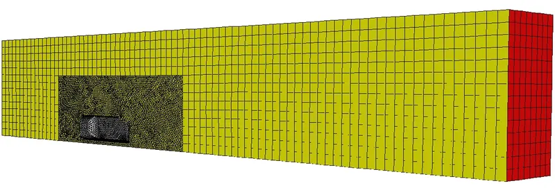
Viscous Model: K-Omega:

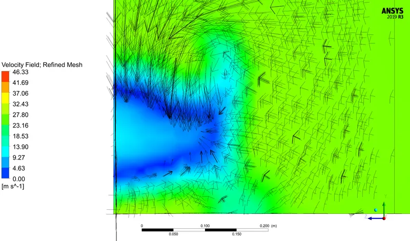
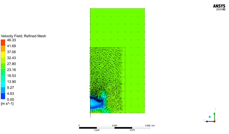
Velocity and Vector Field:

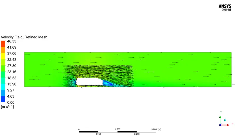
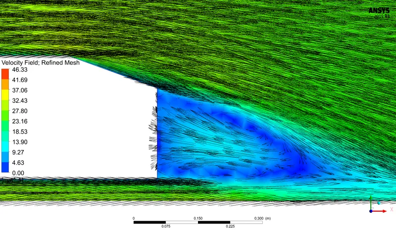
Pressure Field:

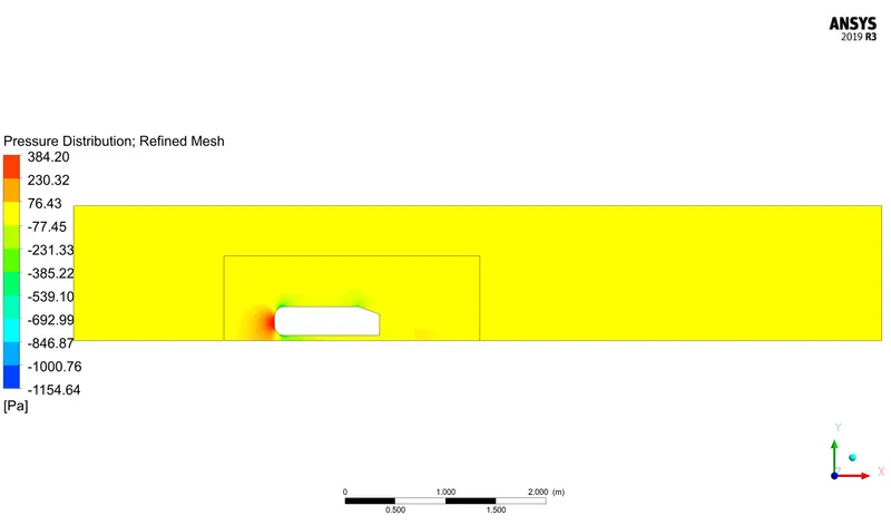
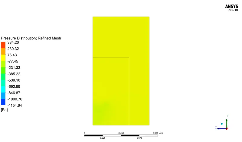
Inference from Contour Plots:

The velocity value behind the Ahmed body drops to around 12m/s to no flow condition. In the velocity vector field, we can clearly notice the boundary separation captured by the added inflation layers, and the air surrounding the Ahmed body in high pressure which is being sucked into the vacuum region. Here in comparison to the previous basic mesh model, the flow field is captured clearly as seen in the vector plot wherein the reverse flow is captured perfectly.

The Pressure contour says the maximum pressure is on the front of the Ahmed body where the impact due to air is more with a value of around 360Pa. The wake region behind Ahmed body has a negative pressure(about -80Pa) which is clearly visible in the cross-section contour plane in the wake region.

Results:

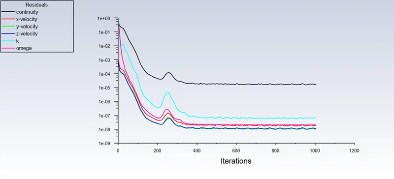
Residual Plot:

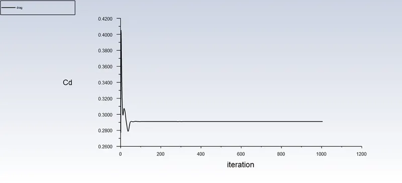
Drag Coefficient Plot:

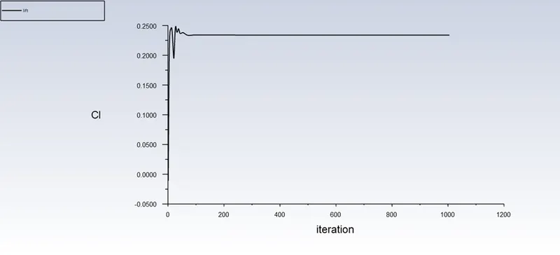
Lift Coefficient Plot:

Inference from Results:

The Residual plot indicates that the simulation has come to an end and the solution has converged. And the coefficient of drag value of 0.29 was recorded. The lift coefficient value was around 0.24
In comparison to the basic mesh model, the drag coefficient value is more accurate here since the flow field parameters are well captured in the wake region.

Refined Mesh Body/Vidcous Model:K-Epsilon:

The same refined mesh body is used but this time for the K-Epsilon viscous model which has a nature of not precisely capturing the near wall shear stresses, but can be used for flow conditions far from the wall.

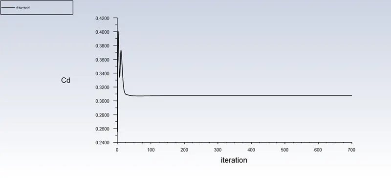
Thus in order to test the accuracy of a different viscous model over the same Ahmed body, we have done the simulation which resulted in the Coefficient of Drag value of 0.31 which is almost accurate.

GRID INDEPENDENCY & VISCOUS MODEL TEST:

The grid independency test was done for two different mesh cases and is compared below.

S.No	Mesh Type	Viscous Model	Cell Count	Coefficient of Drag	Coefficient of Lift
1.	Basic	K-Omega	93171	0.34	0.225
2.	Refined	K-Omega	471553	0.29	0.24
3.	Refined	K-Epsilon	471553	0.31	0.23

CONCLUSION:

The case setup was made only for half of the body and its enclosures using the Split-body command, due to its symmetrical nature, which saved a lot of simulation time. For the common K-Omega viscous model, the drag coefficient value for the Basic mesh model was around 0.34 and that of the Refined mesh model was 0.29. Since both are almost equal and also had their simulation time and iterations to converge equal, we can prefer any type of meshing. But if we need a clear view of the flow field, then we must opt for the refined mesh case. Now, in comparison with the K-Omega and K-Epsilon viscous models for the common refined case, the overall drag coefficient value doesn't make a difference, but if we need to capture the near wall effects clearly then we obviously need to go with the K-Omega viscous model.

Theory Source: Fluid- Dynamic Drag by Sighard F. Hoerner