Week 3 - External flow simulation over an Ahmed body.

Aim:

External flow simulation over an Ahmed body.

Objective:

The objective of this project is to determine the aerodynamic forces that acts on Ahmed body such as drag and lift coefficient and to perform the grid independence test.

The expected results will include

1. Velocity and pressure contours.

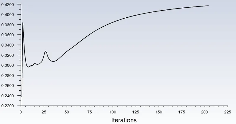
2. The drag coefficient plot for a refined case. ( For a velocity of 25m/sec, the drag coefficient should be around 0.33).

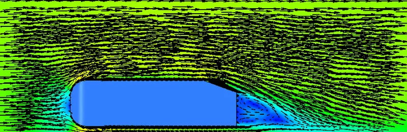
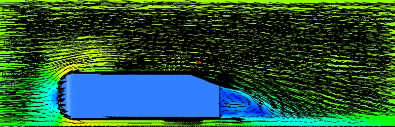
3. The vector plot clearly showing the wake region.

4. Perform the grid independence test and provide the values of drag and lift with each case.

*Ahmed body:

The Ahmed body was first created by S.R. Ahmed. It is an important benchmark for aerodynamic simulation tools. It will be clearly shown in the sketch below that it has a length of 1.044 meters, the height of 0.288 meters and the width of 0.389 meters. It also has a 50 millimeter cylindrical legs attached to the bottom of the body and the rear surface which has a slant that falls of at 35 degrees.

The flow for the model is turbulent which is based on velocity and body length. For the default mesh size in ANSYS-FLUENT we will use K-epsilon model and for the later stage K-Omega SST model is used.

Importance of Ahmed body

The drag force is an important factor considering fuel consumption. As the drag force increases the fuel consumption also increases which in turn affects the car owners economically. As the burning of fossil fuels becomes an issue, the manufacturers focusing pn fuel-efficient cars. One of the main factors considering the car is fuel-efficient or not is the car's geometry because of aerodynamic forces acting on it.

Complex shaped cars are very challenging to model and its difficult to quantify the aerodynamic drag computationally. The Ahmed body is a benchmark model widely used in the automotive industry for validating simulation tools.

*Negative pressure in the wake region

When the air moving over the vehicle is separated at the rear end, it leaves a large low-pressure turbulent region behind the vehicle which is known as the wake. This contributes to the formation of pressure drag which affects the vehicle performance.

When the vehicle is moving at a certain velocity the fluid imparts viscous force to the vehicle as long as it is in the viscous sublayer of the boundary. When the fluid reaches the rear end of the vehicle it gets detached from the surface of the body(which is separation) causing negative pressure in the wake region. The movement of the fluid around the vehicles depends on the geometry of the car and the Reynolds number.

Significance of point of separation

The point of separation will occur when there is a discontinuity in the surface or a region of the negative pressure gradient (a sharp end or rear portion of the car).

When the flow is attached to the body of the vehicle the viscous force will increase which will increase the pressure and a decrease in velocity before the rear end of the vehicle. As soon as the air encounters the sharp turn causing the velocity to decrease resulting in the negative pressure region which is in the wake region. The recirculation region happens beyond the point of separation.

If the rate of change of pressure is large the mixing process will not occur and the boundary layer flow stops.

The flow gets separated from the boundary layer and there is a region of recirculation after which the flow attaches itself to the boundary layer.

In order to reduce the separation of fluid from the boundary layer, it is advisable to have a smooth edge to reduce the effect of drag on the vehicle.

Modeling approach

CASE SETUP IN ANSYS FLUENT:

• Since the Ahmed body is symmetric about the X-Y plane (shown above), the body is to be split into two symmetric half by using split body command in spaceclaim and the 'symmetry' boundary condition is to be applied. This helps to save a lot of computational cells that can be used to further refine the wake region.

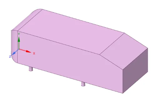
Ahmed Body

• The given problem is external aerodynamic simulation. A wind tunnel is created over the Ahmed body using the ' Enclosure' option in Spaceclaim. This outer enclosure contains a smaller, inner enclosure (for local refinement) which in turn contains the surface of the Ahmed body. While creating the inner enclosures, the 'Interference' option was used to remove any geometric interference and common regions created by the double enclosures. The 'topology' option is set to 'Share' to ensure data is shared between different enclosures for meshes to connect properly.

Outer Enclosure and Inner Enclosure:

• The outer enclosure is of bigger dimensions to make the inflow and outflow boundary conditions not be influenced by the presence of the Ahmed body. But it is impractical to make the whole domain thoroughly refined because it would result in a waste of computational resources. Hence a smaller inner enclosure is created for the purpose of local refinement. It is of immense importance to refine the mesh much more, closer to the geometry, and is shown below.

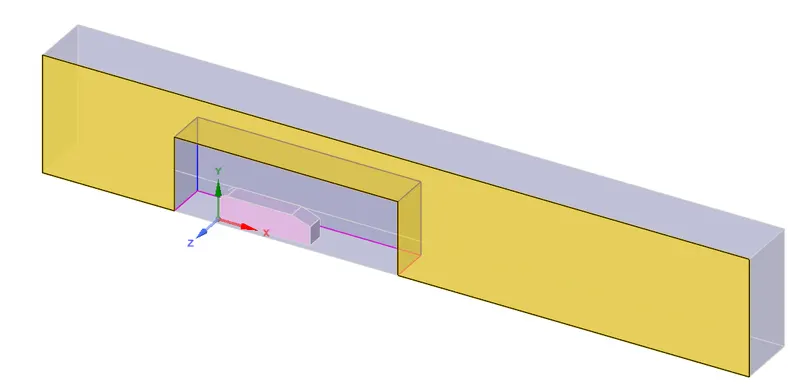
Enclosure after Splitting

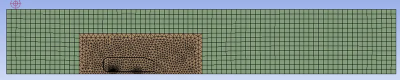
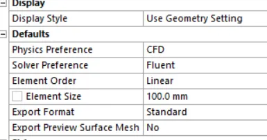
• Next, the Mesh window is opened . Since the geometry of the outer enclosure is made of straight lines, the 'hex' mesh is used.The 'Multizone' mesh method is applied to the outer enclosure to connect between different mesh types. The base mesh size is set to 100mm. The inner enclosure holds the surface of the Ahmed body and hence is 'triangle dominant'.

• The inner enclosure is given 'mesh body sizing' and is set to a size of 30mm. Mesh 'face sizing' with a size of 2mm is given on the cylindrical stands of the Ahmed body to prevent geometry distortion at the stands. To capture the near-wall physics accurately, a boundary layer mesh (Body fitted Mesh) (or) Mesh inflation is provided to the geometry. To come up with the right mesh size, the following calculations are done.

• To capture the near-wall effects, the 'K-omega' SST Turbulence model (y+ range 1 to 5) is preferred. The mesh inflation option is set to 'Total thickness'. Two parameters are required: The total thickness of inflation and the number of inflation layers. Firstly, the boundary layer thickness at the end of the Ahmed body is calculated using the boundary layer formula for turbulent flow over a flat plate. Considering the y+ for the problem as 1, the first layer thickness is calculated.

* Y+ is calculated using Y+ Calculator ,which is available online ' https://www.cadence.com/ko_KR/home/tools/system-analysis/computational-fluid-dynamics/y-plus.html '

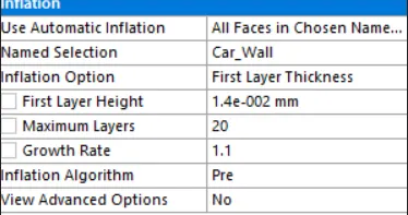
• The number of inflation layers is 10(for k-epsilon base mesh) & 20 (for K-Omega SST). Taking into account the slanted surface at the end of the geometry and the developing vortices, the number of layers is set to 10(for k-epsilon base mesh) & 20 (for K-Omega SST) with a First layer thickness of 0.7mm(for K-epsilon) & 0.014mm(for K-omega SST). With this, the meshing is complete.

• Next, Fluent is opened and a mesh-check is performed. A pressure-based steady-solver is used for the case as the flow speed of 25 m/s is well below Mach 0.3. At the reference values, the projected area, length, velocity, region from which flow occurs are specified. The turbulence model is set to K-epsilon & K-Omega SST for alternate simulations. Material is 'air'. The boundary conditions inlet - veloity inlet , outlet - pressure outlet, wall,domain - symmetry.

• The problem is then initialized using the Hybrid solver. Plots such as coefficient of lift, coefficient of drag, wall shear stress, pressure contours, velocity contours, vector plots are set up before the simulation. Finally, the case is run for 500 iterations.

Results:

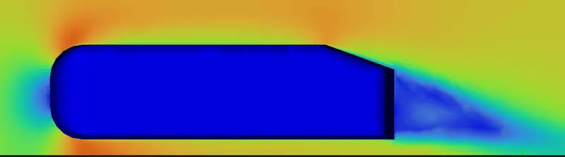
Base mesh:

Velocity and pressure contours:

Velocity:

Pressure:

Cd plot:

Vector plot showing the wake region:

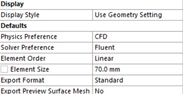
refined mesh with K-epsilon model:

Velocity and pressure contours:

Velocity:

Pressure:

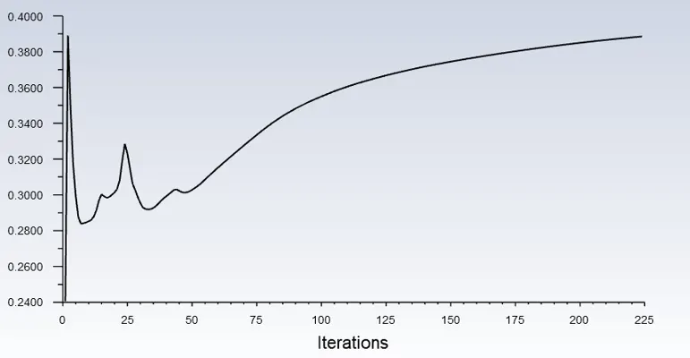
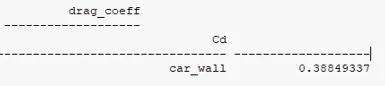
Cd plot:

Vector plot showing the wake region:

With K-Omega SST Turbulence model:

For K-Omega SST model y+ = 1 is preferred in this simuation , calculated first layer thickness as 0.014mm.

Velocity and pressure contours:

Velocity:

Pressure:

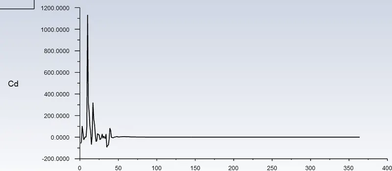
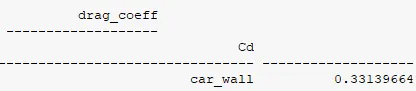
Cd plot:

Vector plot showing the wake region:

Demonstration of grid independence test:

Comparison of all cases

Grid Independence Test	Turbulence-model	Number of elements	Lift-Coefficient	Drag-Coefficient
Baseline mesh	K-epsilon	295659	0.3066280	0.417133
Refined mesh	K-epsilon	399791	0.281555	0.388493
Refined mesh	K-Omega	676971	0.2187788	0.331396

It can be inferred that the imitation of the experimental result is obtained during the refined mesh in K-omega sst model. Thus the grid independence test saves a lot of computational time and convergence can be achieved by using smaller cell sizes for calculation.