Week 3 - External flow simulation over an Ahmed body.
Aim : To simulate the flow over Ahmed body and to plot for velocity and pressure contours, the vector and drag coefficient plot.
Theory :
Ahmed Body :
The Ahmed body represent a simplified vehicle model. This was first developed by SR Ahmed and hence named it as Ahmed body. The airflow around Ahmed body captures the flow features around the automobile. This simplified body is able to capture almost the same airflow which will occur to an exact automibile.
Importance in practical applications :
The Ahmed body is a generic car body (a simplified vehicle model). The airflow around the Ahmed body captures the essential flow features around an automobile and was first defined and characterized in the experimental work of Ahmed. Although it has a very simple shape, Ahmed body allows us to capture characteristic features that are relevant to bodies in the automobile industry. This model is also used to describe the turbulent flow field around a car-like geometry. Once the numerical model in validated, it is used to design new models of the car. Car companies makes numerous attempts to develop modified designs to effectively reduce the aerodynamic drag force which occurs at the rear end without putting any constraints in the stability, comfort and safety of the passengers.
Solving and modelling approach :
A. Geometry
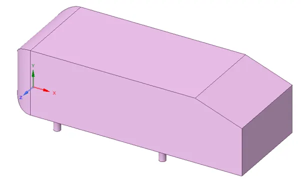
1) Import Ahmed body geometry in the SpaceClaim.
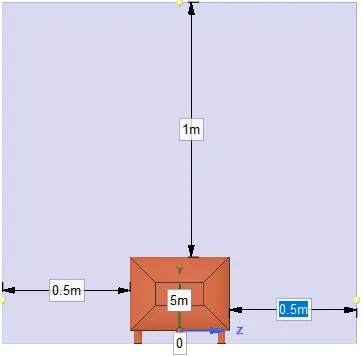
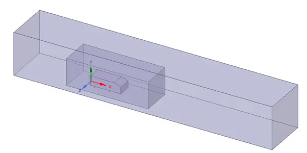
2) Prepare an Enclosure for the Ahmed body
Side view

Front view
3) Add another Enclosure of smaller dimensions.
Side view
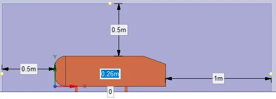
Front view
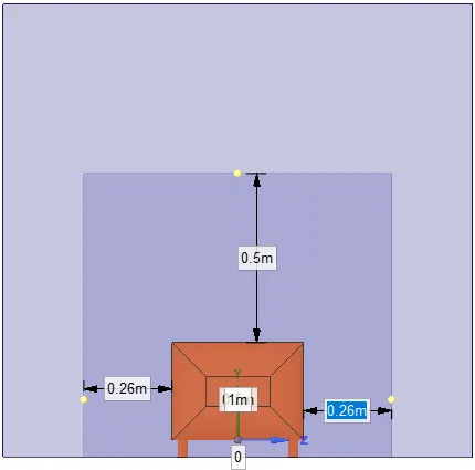
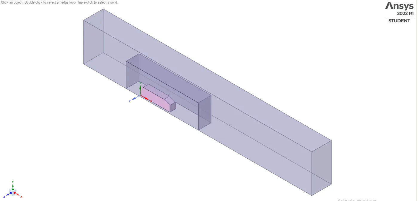
4) Final geometry after adding Enclosures is shown below:
5) Add a plane and view in section mode for the interference.
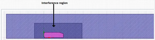
6) In prepare section click on interference it will show interference region.
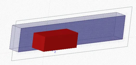
7) Press on green tick and I will resolve the interference problem.
Resolved interference
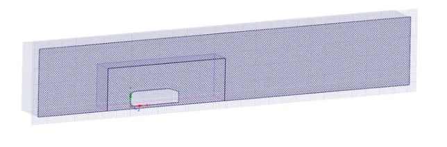
8) Suppress the Ahmed body for physics.
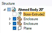
9) Close SpaceClaim.
B. Meshing
1) Open meshing interface and click on generate mesh at default values.
Baseline mesh is show below:
Side view

Bottom surface
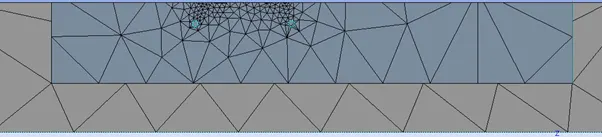
2) Now insert a meshing method and for method use multizone. When we will use multizone it will automatically use hexahedral mesh where ever possible.

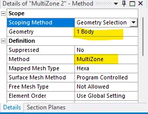
3) Select the outer box and apply in geometry
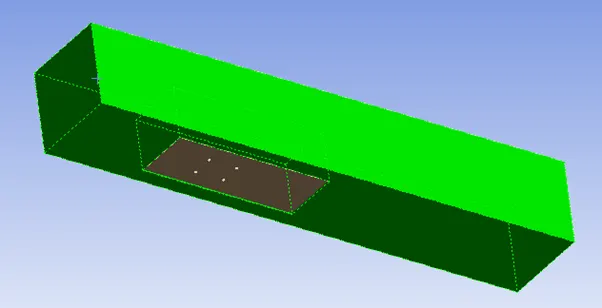
4) Generated mesh for outer box is shown below:

5) Now insert sizing and select inner box as geometry and element size as per requirement and generate mesh.
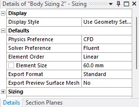
6) Generated mesh is shown below:
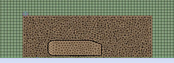
7) Insert sizing and select 4 cylindrical stands of the body for the geometry and apply and set element size as per requirement.
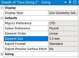
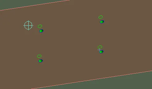
Generated mesh is shown below:
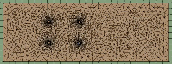
8) Add inflation layer to the car-body surface and select inflation option as First layer thickness.
First layer height is calculated from Y+.
Generated mesh is shown below:
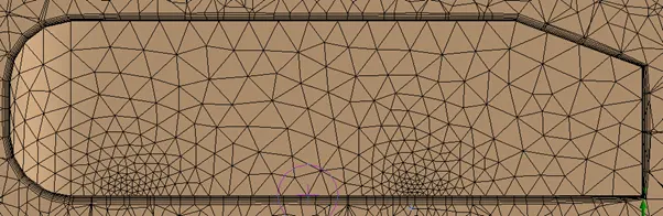
Inflation layers:

9) Close meshing and update the mesh.
C. Setup
1) Open fluent setup and perform mesh check to ensure mesh generated is free from errors.
2) Set Reference values
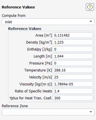
3) Change viscous model to realizable k-epsilon model and chose standard wall function.
4) Add material type as fluid and material air.
5) Change boundary conditions
Inlet velocity = 25 m/s
6) Now perform hybrid initialization.
7) Create a definition for drag coefficient.Similarly create definition for lift coefficient.
8) Create a velocity and pressure contour at cut-plane.
9) Run calculation.
Case 1 : Baseline setup
In baseline setup outer enclosure is created in spaceclaim and model is meshed using default mesh size.
Meshed model is setup is done in Ansys-fluent and calculations are done.
We get following results;
Residuals :
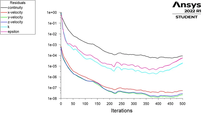
Drag coefficient :
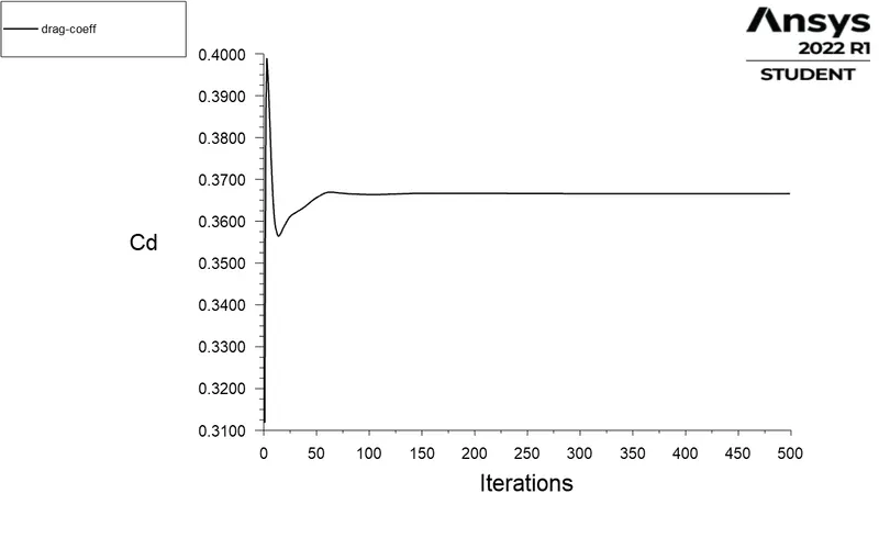
Computed Cd = 0.3666
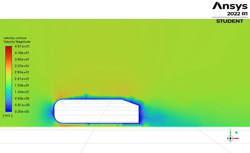
Velocity contour :
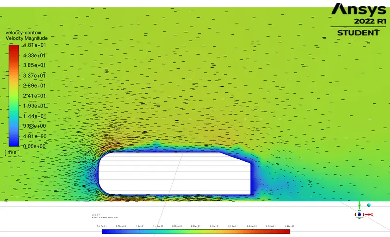
Vector plot :
Observations :
- The results are very coarse as we use the default mesh size we need to improve the mesh quality.
- The velocity not captured good we need to do refinement to get accurate results.
- The computed Cd = 0.3666 which is calculted using default mesh size and without refinement.
To get more accurate results we need to improve the meshing. The region of refinement is given just before the Ahmed body lets called it inside enclosure.
Case 2 : Refined setup
Outer and inner enclosures are created in spaceclaim. Inner enclosure is created such as it will capture the wake region.
Outer enclosure is meshed using multizones and hexa elements of element size = 100 mm are created.
To perform the grid independency test the inner enclosure is meshed using different mesh sizes such as,
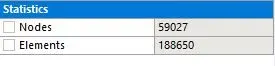
A) Mesh size = 50 mm
B) Mesh size = 40 mm
C) Mesh size = 30 mm
A) Mesh size = 50 mm
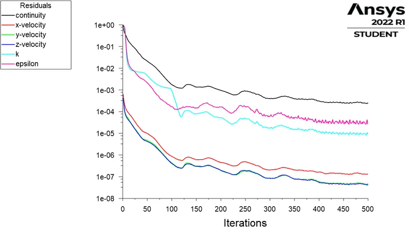
Residuals :
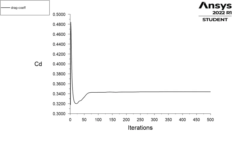
Drag coefficient :
Cd = 0.3439
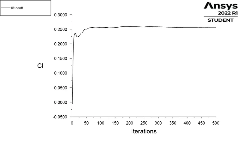
Lift coefficient :
Cl = 0.2565
Velocity contour :
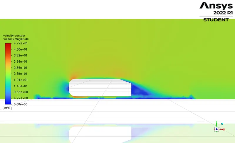
Velocity contours shows the velocity distribution around the body and within the computional domain.
Pressure Contour :
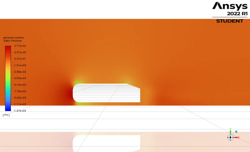
Pressure contours shows the pressure distribution over a ahmed body and within the computional domain.
Vector plot :
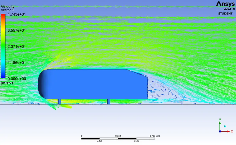
Vector plot shows the flow direction of velocity vectors.
All of the required physics i.e wake region is captured in this case but still we cant be sure with obtained drag and lift cofficient values thus to see the effect of refinement on obtained results we go for second refinement.
B) Mesh size = 40 mm
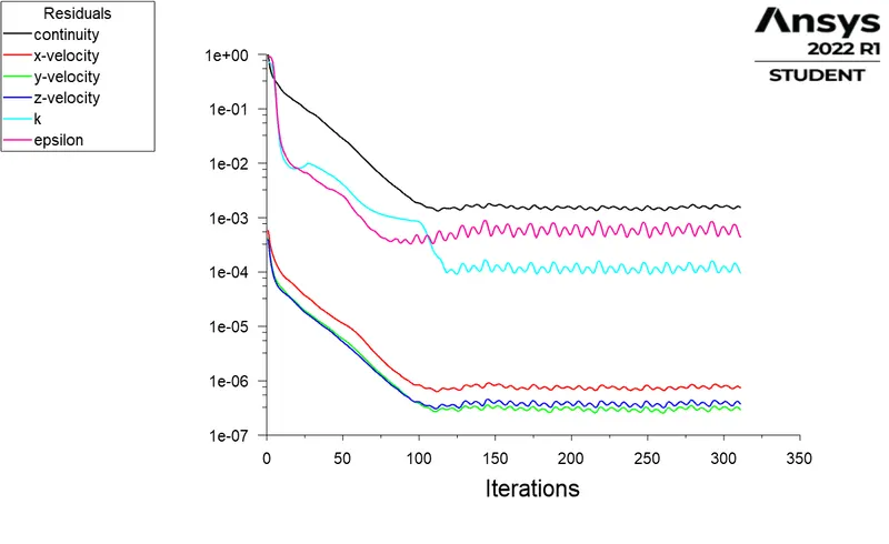
Residuals :
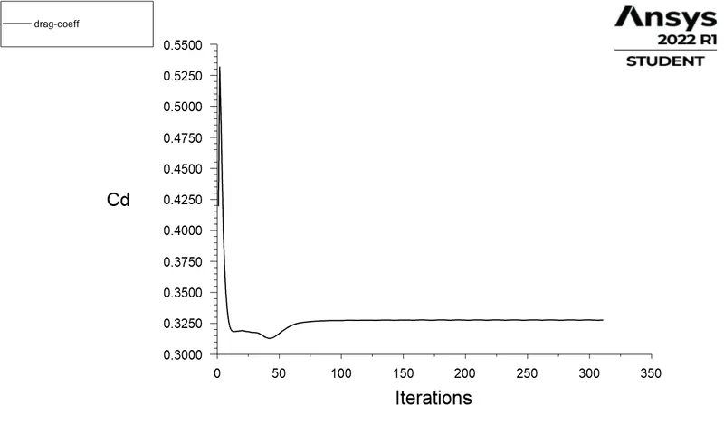
Drag coefficient :
Cd =0.3277
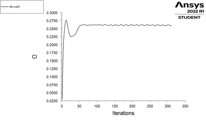
Lift coefficient :
Cl = 0.2594
Velocity contour :
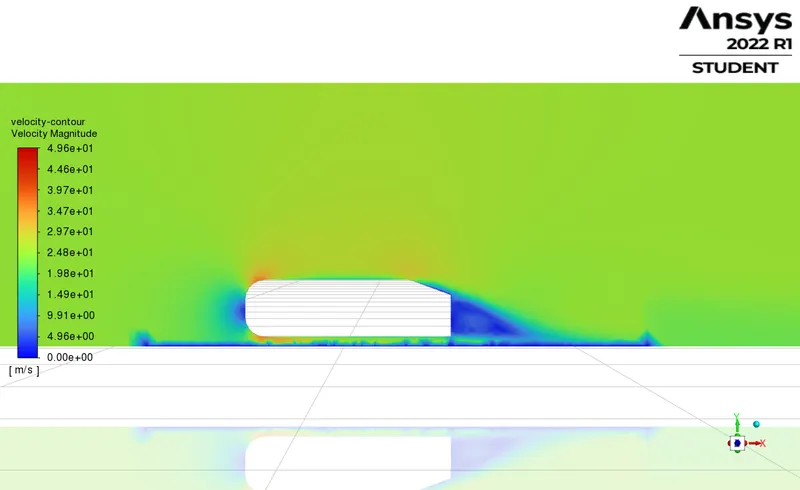
Velocity contours shows the velocity distribution around the body and within the computional domain.
Pressure Contour :
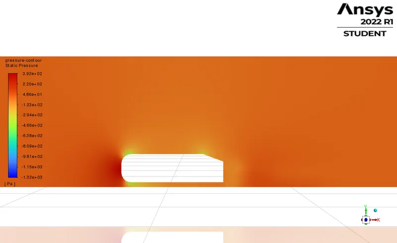
Pressure contours shows the pressure distribution over a ahmed body and within the computional domain.
Vector plot :
Vector plot shows the flow direction of velocity vectors.
Thus the results of drag cofficient and lift cofficient is varried from 1st case to second case. Lets see the the effect on results on further refinement.
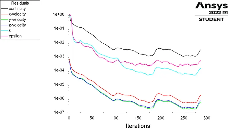
C) Mesh size = 30 mm
Residuals :
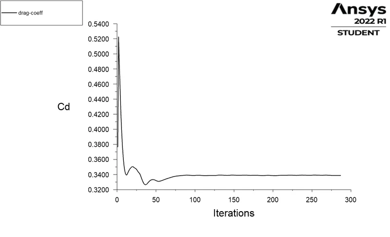
Drag coefficient :
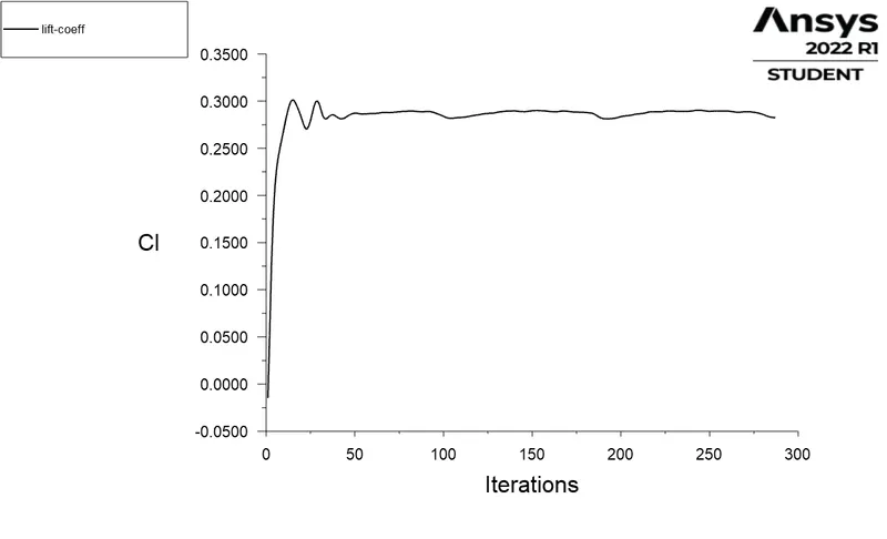
Cd = 0.3387
Lift coefficient :
Cl = 0.2823
Velocity contour :
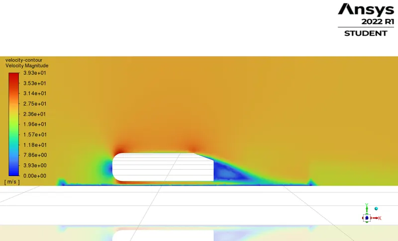
Velocity contours shows the velocity distribution around the body and within the computional domain.
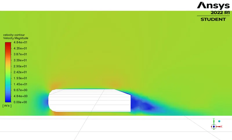
If we compare this case velocity contours with other two case then we can see that the wake region shown in this case has a more definite shape than other two cases and this is due to highly refined mesh.
Pressure Contour :
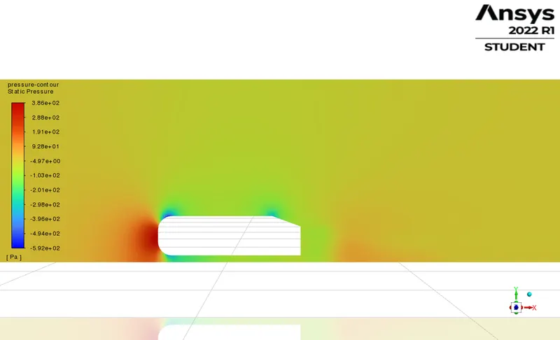
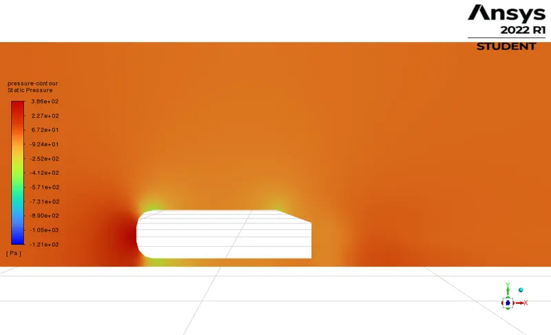
The frontal region of Ahmed body is flow impacting region which generates high static pressure. In this case the impacted region and negative pressure region can be seen accurately.
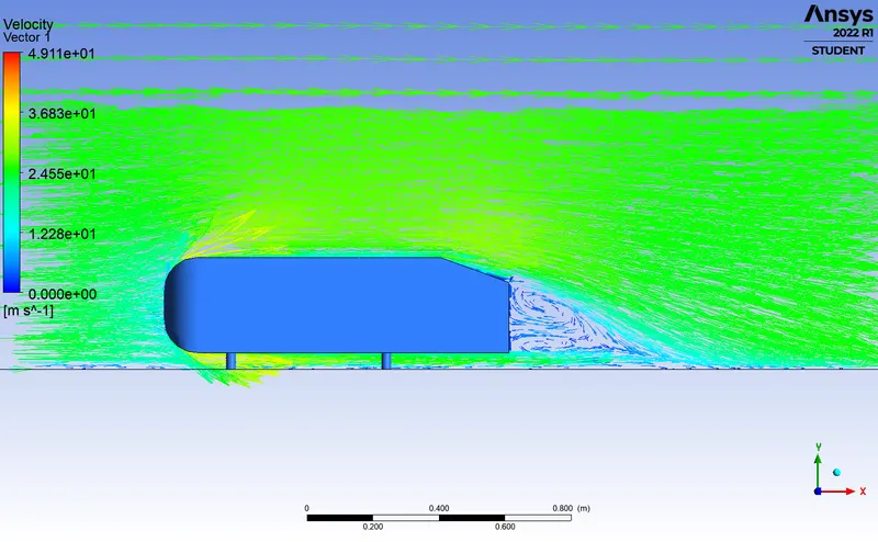
Vector plot :
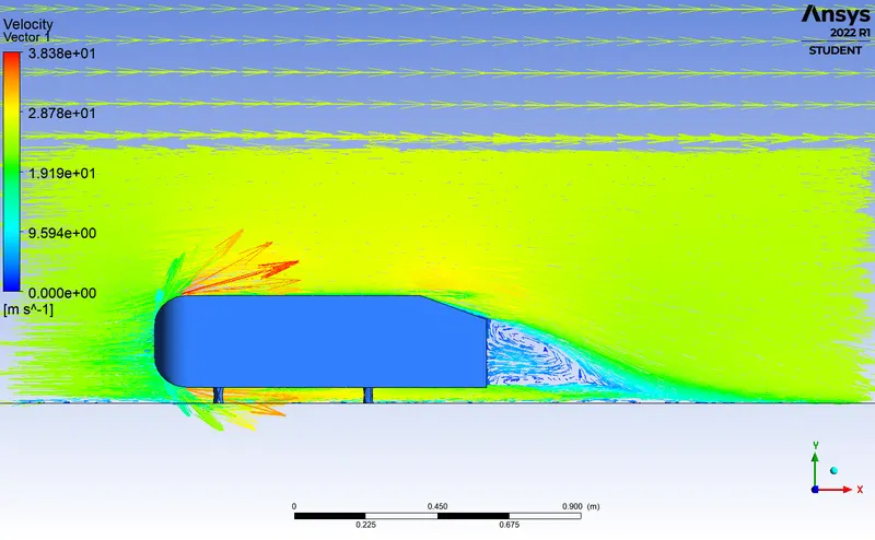
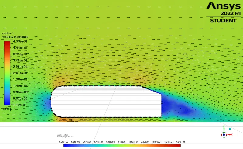
The vector plot clearly shows that the recirculated region is formed behind the ahmed body which has low velocity and the air is forming eddies behind the ahmed body.
As the body is perfectly symmetric, we can run the simulation by considering the only half body. This is the best practice where you can save on the number of cells and get the results faster as well.
Case 3 : Half Ahmed body
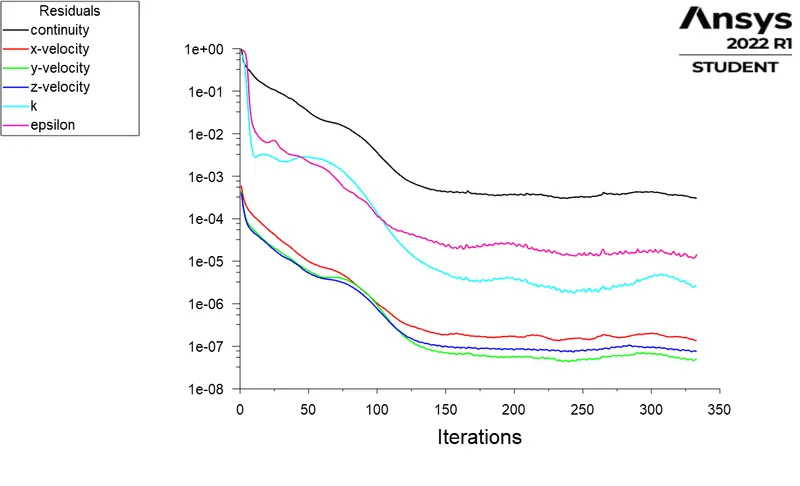
Residuals :
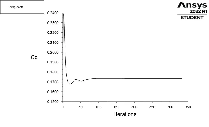
Drag coefficient :
Cd = 0.1733
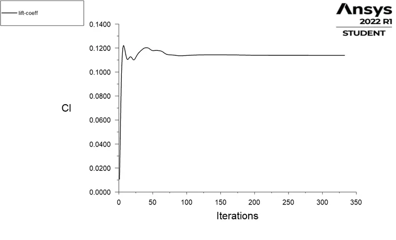
Lift coefficient :
Cl = 0.1138
Velocity contour :
Pressure Contour :
Vector plot :
Negative pressure in the wake region :
We observed that a wake region(a large recirculation region) have established at the rear side of Ahmed body in velocity flow Which have created a vortex flow at rear side.
When the air moving over the vehicle is separated at the rear end, it leaves a large low pressure turbulent region behind the vehicle known as the wake. This wake contributes to the formation of pressure drag, which is eventually reduces the vehicle performance.
Formation of recirculation zone is also one of the reson for formation of negative pressure in a wake region.
The negative pressure in the wake region can be releated to the recirculation region caused after the bluff body. As the air hits the frontal area of the Ahmed body it is subjected to a high pressure region which is termed as stagnation point. Since vehicles can be treated as a bluff body, the flow will experience seperation at the rear leading to wake region behind the body. This is the main reson for aerodynamics resistrance.
Point of Seperation :
Separation of flow is said to occur when the direction of the flow velocity near the surface is opposed to the direction of the free stream velocity, which means `(du)/(dy)<=0`. Here the skin friction coefficeient reaches to a vlue of zero. At this point the wall shear stress vanishes and is called the point of seperation. Reverse flow take place beyond this point. due to reverse flow large eddies are formed and a lot of energy is dissipated. this region is inturn called as wake.
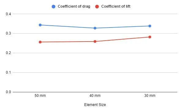
Grid independance Study :
| Element Size (mm) | No. of elements | Coefficient of drag | Coefficient of lift |
| 50 | 188650 | 0.3439 | 0.2565 |
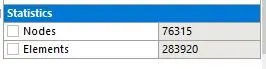
| 40 | 283920 | 0.3277 | 0.2594 |
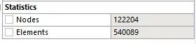
| 30 | 540089 | 0.3387 | 0.2823 |
Conclusion :
Refining the mesh defenitly increases the quality of results, being an acadamic version of ansys the no. of elements was limited on to 0.5 million cells which restricts the quality of results. The element size = 40 mm showed a coefficicnet of drag 0.3277 for 25m/s velocity.
The grid dependency test allows us to see smoother velocity profile. As we make the mesh finer i.e. when we increase the cell counts (closer to the limit), we can see from the vector plots from all the 3 cases, of the velocity that it becomes more and more smoother. One thing is observable that making the mesh finer lets us see the wake region more prominent. From the 3 cases, we can conclude that the flow is more defined at lower element size i.e. at case 3. The finer the mesh gets, the easier it gets in visualizing the contours. Mesh refinement increases the closeness of the resulting values to the true values.
The graphical plots and contours for all three types of mesh are almost the same. Small differences are noticed in the appearance of the plots and contours but that is due to the difference in element quality. If we notice the velocity contour then we can see that the velocity around the wake region is high and low at the tail of the Ahmed body. If we connect this observation with the velocity vector plot then we notice that at the wake region the velocity vectors are large which is obvious due to the obstruction offered by the Ahmed body and at the tail of the body there is a circulating flow which is the reason for its low velocity. Whereas, for the pressure contours at the car wall and XY plane, high pressures are observed in the front of the body, and in the wake region we observe negative pressure.