Week 3 - External flow simulation over an Ahmed body.

1. Background:

the movement of air over the roof of the car is separated at the end of the roof; a phenomenon is known as the wake. The wake is a low-pressure zone and its location is behind the car. The shape of the rear of the car is more important than the shape of the front because of the wake.

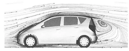
Figure 1.1: Flow visualization by computer simulation

1.1 Different rear end shapes:

Reynolds Averaged Navier-Stokes (RANS) was used to calculate drag coefficients.

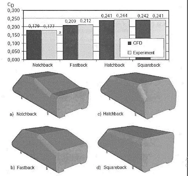
Figure 1.2: The four types of rear-end shapes of road vehicles with measured and simulated drag coefficients

S.No.	Type	Application
a.	Notchback	Family car. the most streamlined shape.
b.	Fastback	Supercar, sports car. The wake area is small.
c.	Hatchback	Small family car.
d.	Squareback	station wagons, Sport Utility Vehicles (SUVs), vans and buses. The wake area for this type of design is large.

Figure 1.3 shows the effect of the shape of the front and rear of the vehicle in Lay’s study of 1933. Obviously, the rear end shape of the vehicle has a greater influence on the drag coefficient.

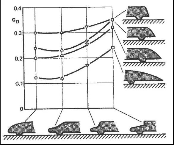
Figure 1.3: Summary of the test results by Lay

This study focuses on the aerodynamic behaviour of road vehicles. Automotive aerodynamic studies started by using simplified models such as the Ahmed model.

Figure 1.4 illustrates the standard geometry of the Ahmed model and its dimensions. Ahmed created this geometry in 1984 and it has become a benchmark to study the main features of aerodynamic behaviour for road vehicles. The Ahmed model is also used to study the behaviour of turbulent flow around simple car geometry.

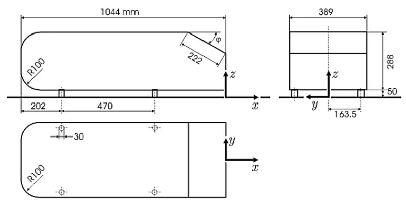
Figure1.4: Standard geometry of the Ahmed model

Q.1. Ahmed's body and its importance: The Ahmed model is simple and free from all kinds of accessories as well as wheels; nevertheless it can be used to study the aerodynamic behaviour of a road vehicle based on the main features such as the slanting surfaces. This model is primarily designed to study the effect the slant angle (α) at the end part of the model on the drag coefficient and vortices behind the vehicle.

Q.2 reason for the negative pressure in the wake region:

pathlines tell us the exact circular motion or vorticity generated just at the rear end of the car. the separation takes two regions of distribution. one at the upper part of rear-end and the other is the lower part of the rear end. the fluid particle away from the rear region having higher pressure besides the wake region try to approach from high-pressure region to low-pressure region thus creating a circulatory wake region.

Q.3 Explain the significance of the point of separation:

Flow separation is responsible for wake formation. The fluid particles decelerate on the front of the cylinder and the pressure increases in this area. The point on the left-hand of the cylinder (forward stagnation point as in Figure 3.3) is called the stagnation point (the flow velocity of this point is locally zero) and is the point of maximum pressure. The thickness of the boundary layer is smallest at the stagnation point and it increases towards flow.

The fluid particles accelerate over the left-hand section of the cylinder, and reach the maximum velocity is in the middle section of the cylinder (point C). When the velocity is a maximum, pressure is a minimum (point C).

the pressure gradient is positive on the backside of the cylinder. The reduction of velocity in this area is due to viscosity and the positive gradient in pressure [70]. The boundary layer flow is retarded, particularly near the body surface, and reversed flow may happen due to a pressure increase in the flow direction. This phenomenon is called separation.

The condition for the separation point D is `((du)/(dy))_(wall)=0`

beyond the separation point, the flow gets back reverse i.e positive pressure gradient along the x-direction is called an adverse pressure gradient.

Favourable conditions: negative pressure gradient(dp/dx), positive velocity gradient(du/dy)

Adverse conditions: positive pressure gradient(dp/dx), negative velocity gradient(du/dy)

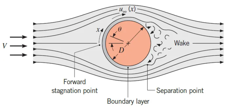
Figure 3.1: Separation on a cylinder in crossflow

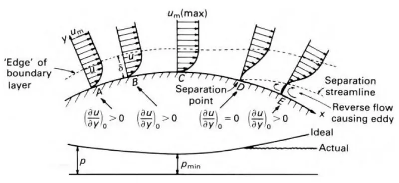
Figure3.2: Flow in the boundary layer on a cylinder before and after the point of separation

Drag coefficient `C_D=(2F_D)/(rhoAV^2); C_L=(2F_L)/(rhoAV^2)`

`R_e=(rhoVL)/mu`

`rhoV=(mu R_e)/L`

`C_D=(2LF_D)/(muR_eVA)=f(R_e)`

drag coefficient will decrease with increase reynold number.

There are five sequential steps to complete this challange.

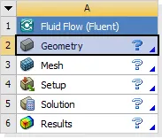
1. Geometry: we open the SpaceClaim by double click on the "Geometry" icon. now import the full-scale geometry model to SpaceClaim from where we have saved the geometry file. the dimensions of the imported geometry model are the same as in figure 1.4 and its units are in millimetres.

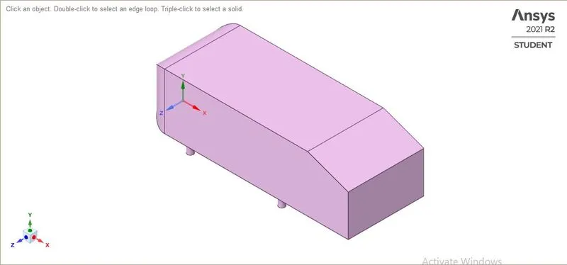
now we change the unit from mm to meter. to simulate the flow over Ahmed's body, first, we create the enclosure or box that will cover the Ahmed body.

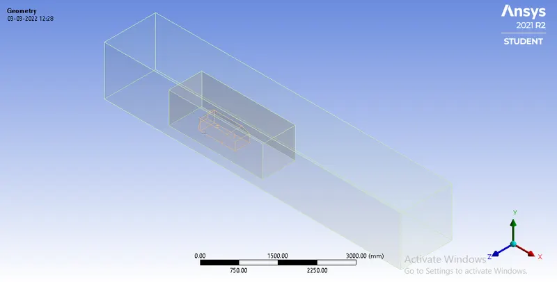
created 2 enclosures. enclosures are created to capture the wake. then after will create 3 perpendicular planes which pass through the reference point. among the 3 planes, we select the vertical plane only then use the cut section tool to see inside the box.

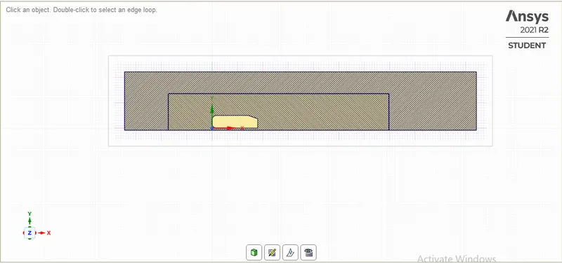
here geometry section has been completed. now will go to the mesh section

2. Mesh:

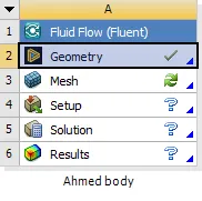
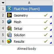
now we do double click on the Mesh section in the workbench. here we define the boundaries by name like inlet, outlet, symmetry and car wall. then click on generate the mesh.

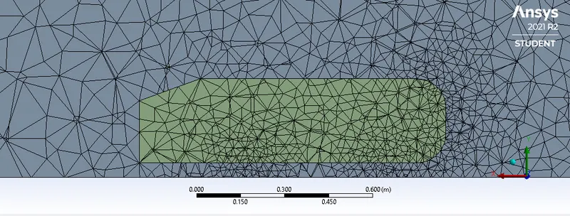
in the above figure, meshing has been done on Ahmed's body also. but we don't want mesh on Ahmed's body because fluid flows over the surface of the body not inside. so first we suppress the physics of Ahmed's body. and select share topology to flow the information from the outer box to the inner box. in the above figure there is a mesh overlap between the outer and inner box.

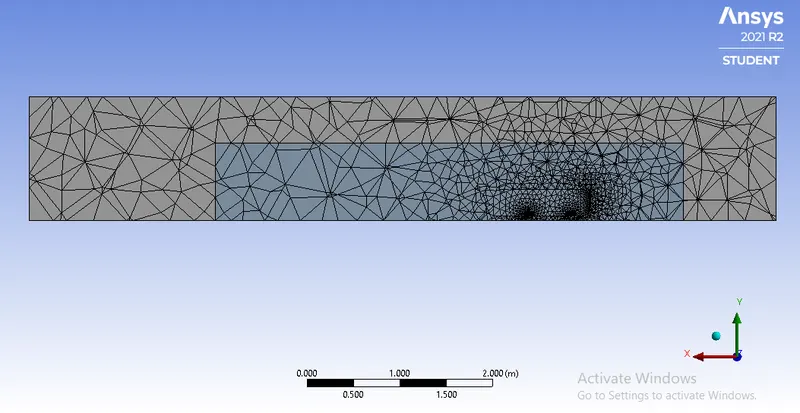
now in the above figure, there is no mesh overlapping which means the information will flow from the outer box to the inner box in a proper way.

Given: fluid velocity, u=25 m/s

Sonic speed, C=342 m/s

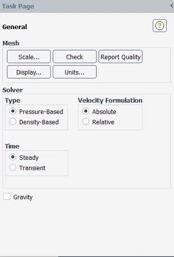
Mach number, M=25/342=0.07(Which is less than 0.3. hence we will use pressure based solver)

`R_e=(rho.V.L)/mu=(1.225times25times1.04)/(1.7894times10^-5)=1,779,926.232`(it is a turbulent flow because the condition is flow over flate plate, Re>5*10^5)

For external flow, `C_f=0.058R_e^-0.2=3.2609times10^-3`

Wall shear stress, `tau_w=(1/2).C_f .rho.U^2=1.2483 N`

Shear velocity, `U_t=sqrt(tau_w/rho)=1.009 m/s`

`Y+=(rho.U_t.Deltay_1)/mu`

Undesirable value of Y+ is between 10 and 30

Desirable values of Y+ are either less than 10 or greater than 30.

so I take Y+=30.

`30=(1.225times1.009timesDeltay_1)/(1.7894times10^-5)`

`Deltay_1=4.34times10^-4 m=0.434 mm`

use multizone and in sizing choose element size 100 mm and maximum element size is 100 to generate hexahedral mesh on the outer box. hence we will get evenly sized mesh(hexahedral) on the outer box.

Case 1:

Outer encloser element size=100 mm

Inner enclosure element size=50 mm

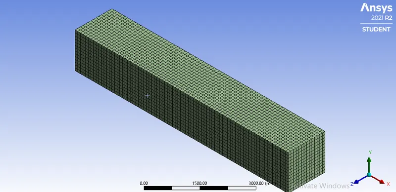
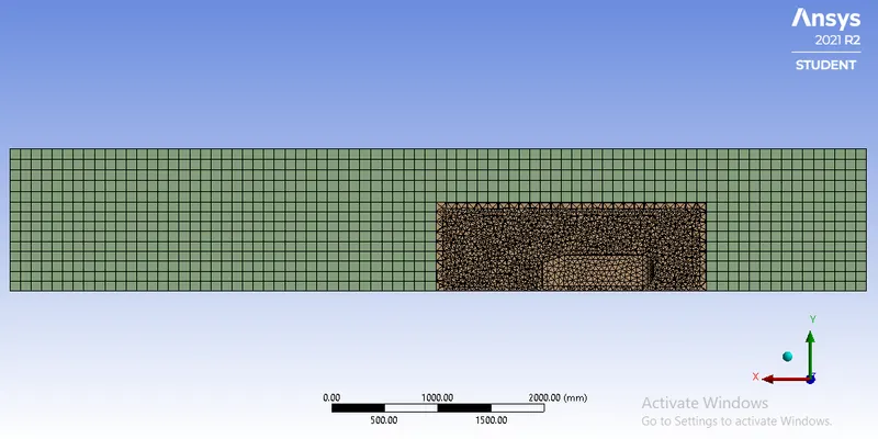
Figure: Cut section

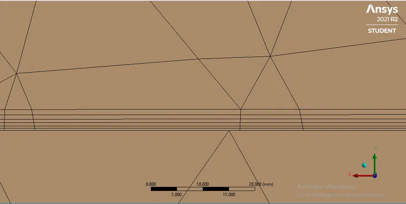
Figure: Inflation layers

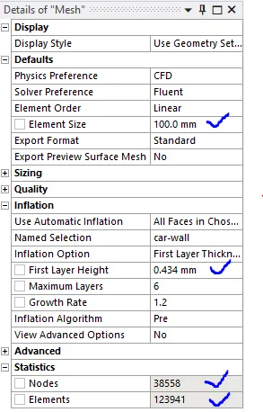
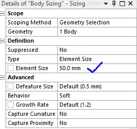
Meshing step has completed. now will click on to setup.

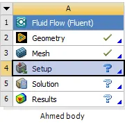
Setup:

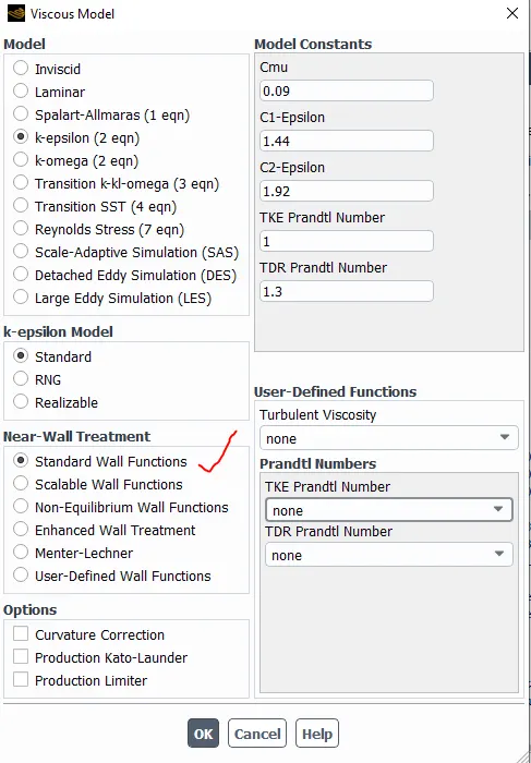
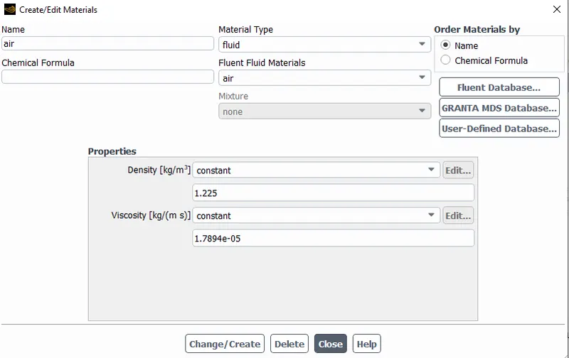
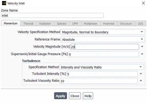
Solutions:

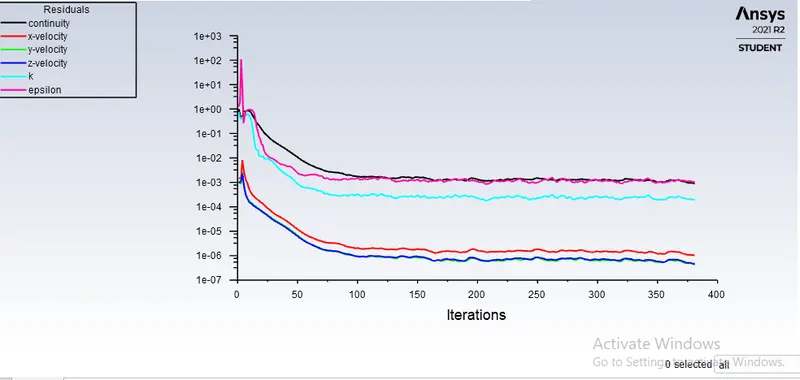
Figure: Residual of the conservation equations applied on the domain for 500 iterations

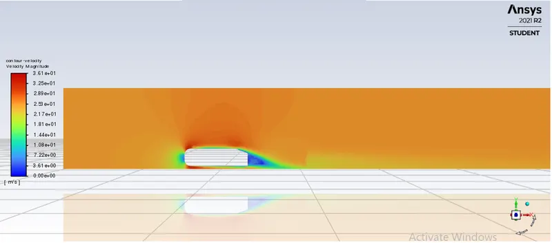
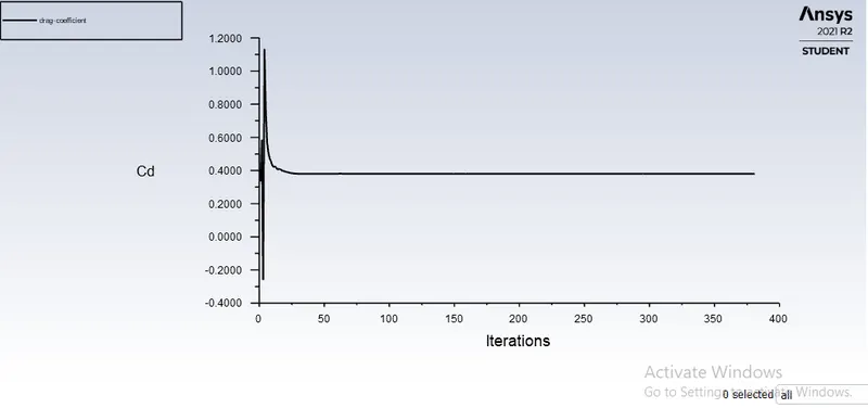
Cd= 0.38017744

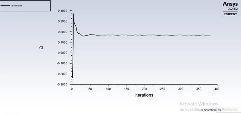
Cl=0.16830331

Result:

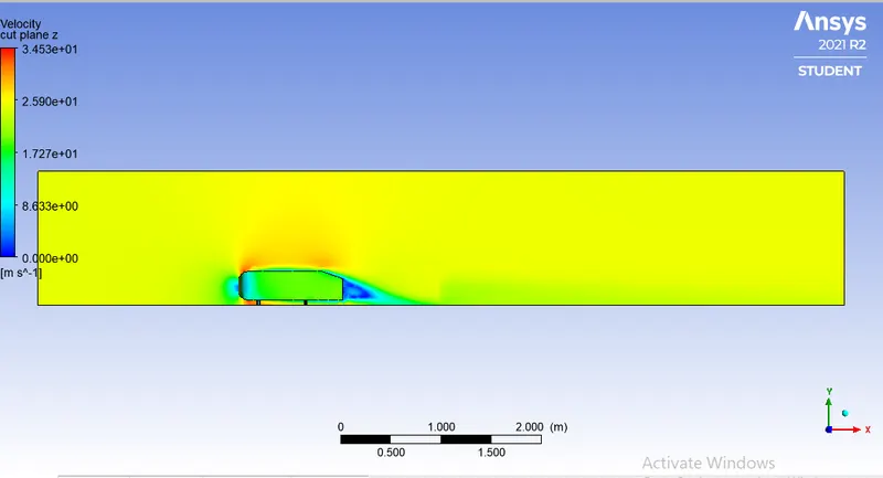
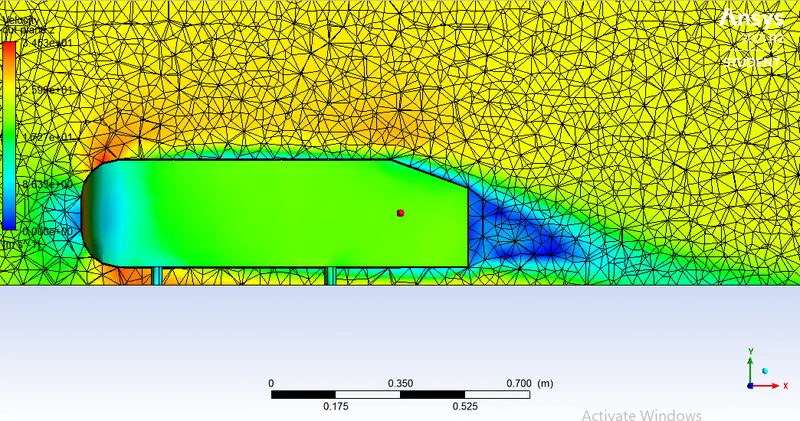
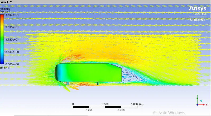
Figure: Vector plot

now draw the velocity profile on a lines which are at different locations on rear side of Ahmed body. and we will see how the velocity changes along a particular line.

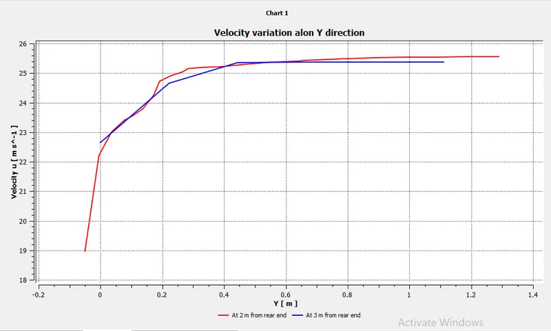
Case 2: outer enclosure element size=90 mm

Inner enclosure element size= 40 mm

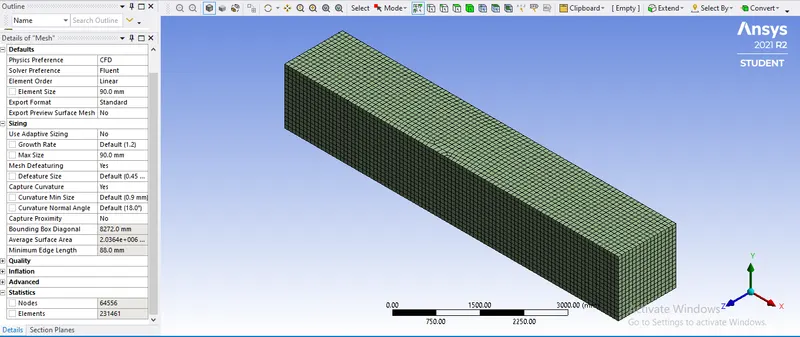
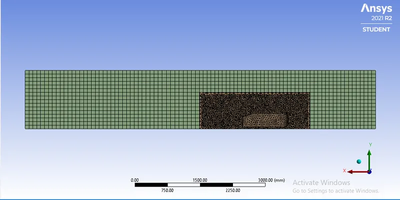
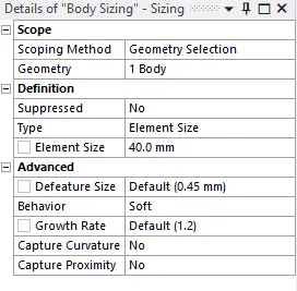
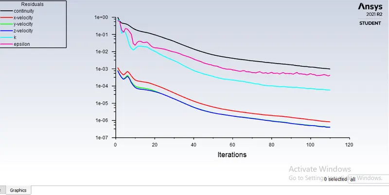
Figure: Residual of the conservation equations applied on the domain for 500 iterations

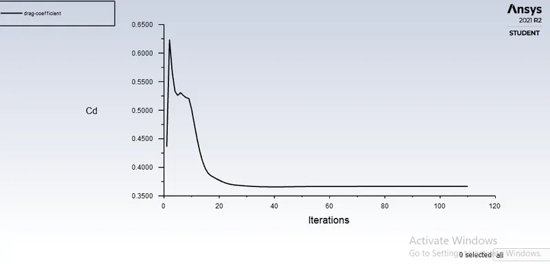
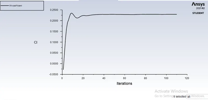
Results:

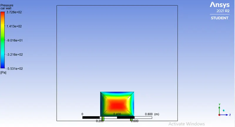
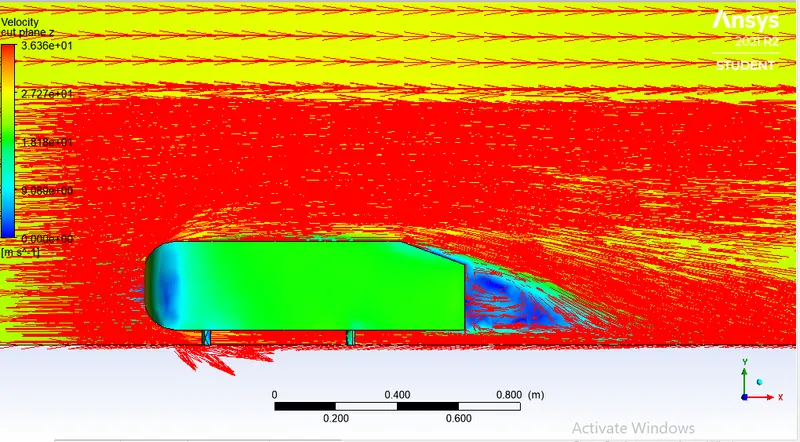
Figure: Vector plot

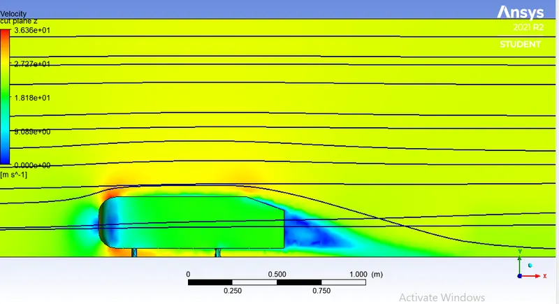
Figure: Streamline plot

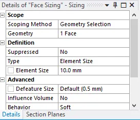
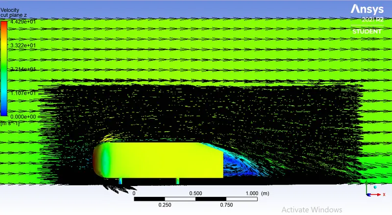
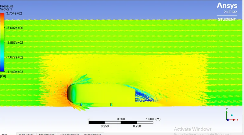
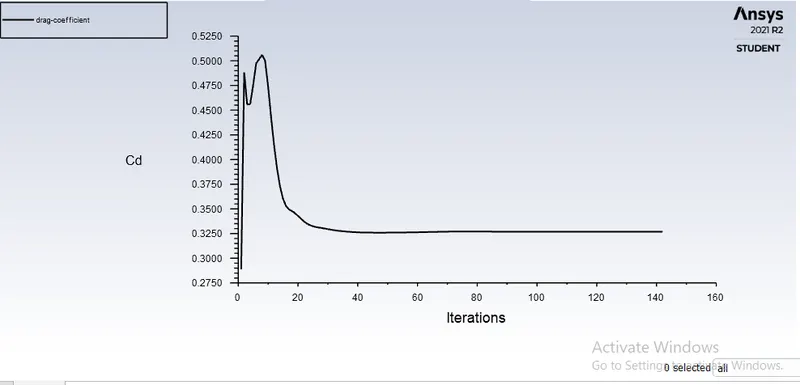
Case 3: Face size(element size)=10 mm

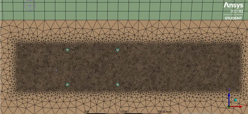
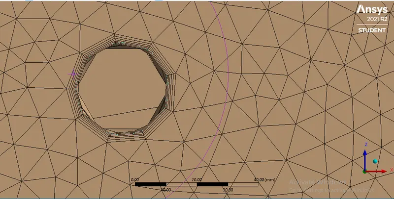
Result:

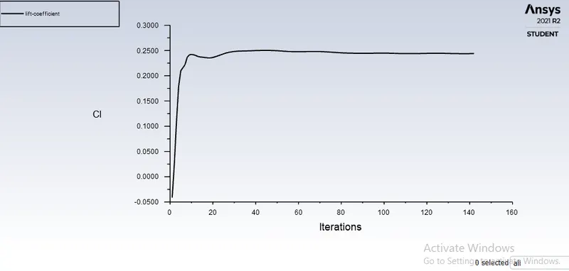
Grid independency test:

To ensure that the mesh size has minimum effect on the final results, a mesh independent study has been carried out. . The number of volume cells is changed in two different runs 123941,231461. The third run with a very fine mesh of 458396 cells is then carried out. The drag coefficient for each run has been calculated

(I have a student version of Ansys software. thereby cant perform grid independency test beyond 512000 cells.)

Name	Case(Run) 1	Case(Run) 2	Case(Run) 3 (here we are changing only face size)
Outer enclosure (element size in mm)	100	90	90
Inner enclosure (element size in mm)	50	40	40
First layer thickness (in mm)	0.434	0.434	0.434
Number of layers	6	6	6
Total thickness (in mm)
Total nodes	38558	64556	113175
Total elements	123941	231461	458396
Drag coefficient	0.38017744	0.36674369	0.32681732
Lift coefficient	0.16830331	0.22927319	0.243887

Conclusion:

1. Initially calculated drag coefficient values are 0.38017744, 0.36674369 which are larger than the acceptable level(0.33)

2. Drag coefficient value decreases with decreasing the element size or meshes size and reaches the experimental value of 0.33.

3. Lift coefficient value increases with decreasing mesh size.