Week 3 - External flow simulation over an Ahmed body.
OBJECTIVE –
To perform external flow simulation over Ahmed Body.
To perform the grid independence test and to provide the values of coefficient of lift and drag.
THEORY –
Ahmed Body - The Ahmed body is a generic car body (a simplified vehicle model). The airflow around the Ahmed body captures the essential flow features around an automobile and was first defined and characterized in the experimental work of Ahmed. Although it has a very simple shape, Ahmed body allows us to capture characteristic features that are relevant to bodies in the automobile industry. This model is also used to describe the turbulent flow field around a car-like geometry. Once the numerical model is validated, it is used to design new models of the car. The rear part of Ahmed body is called a 'slant angle' which influences drag and lift with its critical slant angle which is around 0-40 degrees.
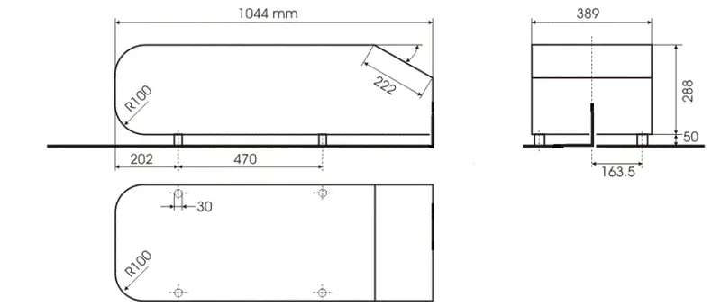
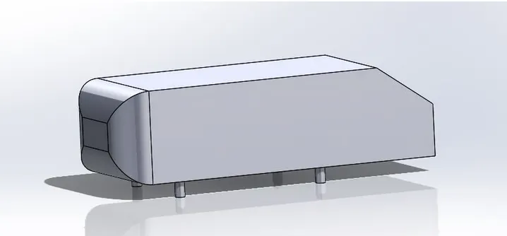
The simple geometrical shape has a length of 1.044 m, a height of 0.288 m, and a width of 0.389 m. It also has 0.5 m cylindrical legs attached to the bottom of the body and the rear surface has a slant that falls off at 40 degrees.
Importance of Ahmed body -
The three-dimensional flow around a vehicle has become a subject of significant importance in the automotive industry. One apparent technique of improving the fuel efficiency of vehicles is to reduce aerodynamic drag force by optimizing the body shape. Execution of fine aerodynamic design under stylistic constraints requires an immense understanding of the flow pattern phenomena and, especially, how the aerodynamics are impacted by changes in body shape. The flow area which presents the major contribution to cars drag is the wake flow backing the vehicle. The point at which the flow separates direct the size of the separation zone, and as a result the drag force. Clearly, a more accurate simulation of the wake flow.
Most cars have an average drag coefficient of between 30 and.35. Boxy cars have a higher number, like the HUMMER H2 vehicle at.57, while more streamlined and agile cars have a lower number, like the Mercedes-Benz C-Class® vehicle at.24. Again, this is just an average measurement. The exact drag coefficient of a car varies with the Reynolds number and various other factors.
Co-efficient of drag -
In fluid dynamics, the drag coefficient (Cd) is a dimensionless quantity that is used to quantify the drag or resistance of an object in a fluid environment, such as air or water. It is used in the drag equation in which a lower drag coefficient indicates the object will have a less aerodynamic or hydrodynamic drag. The drag coefficient is always associated with a particular surface area.
The drag coefficient of any object comprises the effects of the two basic contributors to fluid dynamic drag: skin friction and form drag. The drag coefficient of a lifting airfoil or hydrofoil also includes the effects of lift-induced drag. The drag coefficient of a complete structure such as an aircraft also includes the effects of interference drag.
The drag coefficient (Cd) is defined as
`C_d=(2.F_d)/(ρu^2A)`
where:
Fd is the drag force, which is by definition the force component in the direction of the flow velocity.
ρ is the mass density of the fluid,
u is the flow speed of the object relative to the fluid,
A is the reference area.
Negative Pressure at the wake -
When the vehicle is moving at a certain velocity, the viscous effects in the fluid are restricted to a thin layer called the boundary layer (Outside the boundary layer is the inviscid flow). As thousands and even millions of air molecules draw near the car's front, they start compressing, thus raising the air pressure on the front of the vehicle. Likewise, the air molecules that are travelling along the car's sides are at atmospheric pressure. This means the pressure is lower than the molecules on the vehicle's front. i.e., the fluid flow imposes pressure force on the boundary layer.
When the air reaches the rear part of the vehicle, the fluid gets detached. Within the boundary layer, the movement of the fluid is totally governed by the viscous effects of the fluid. The fluid moving around the vehicle is dependent on the shape of the vehicle and the Reynolds number.
There is another important phenomenon, which affects the flow of the car and the performance of the vehicle. This phenomenon is commonly known as the Wake of the vehicle. When the air moving over the vehicle is separated at the rear end, it leaves a large low-pressure turbulent region (vacuum) behind the vehicle known as the wake. This wake contributes to the formation of pressure drag, which eventually reduces the vehicle performance.
Flow Separation -
Whenever there is relative movement between a fluid and a solid surface, whether externally round a body or internally in an enclosed passage, a boundary layer exists with viscous forces present in the layer of fluid close to the surface. Boundary layers can be either laminar or turbulent. A reasonable assessment of whether the boundary layer will be laminar or turbulent can be made by calculating the Reynolds number of the local flow conditions.
Flow separation or boundary layer separation is the detachment of a boundary layer from a surface into the wake region. Separation occurs in the flow that is slowing down, with pressure increasing, after passing the thickest part of a streamlined body or passing through a widening passage, for example.
Flowing against an increasing pressure is known as flowing in an adverse pressure gradient. The boundary layer separates when it has travelled far enough in an adverse pressure gradient that the speed of the boundary layer relative to the surface has stopped and reversed direction. The flow becomes detached from the surface and instead takes the forms of eddies and vortices.
Y+ concept -
The behaviour of the flow near the wall is a complicated phenomenon and to distinguish the different regions near the wall the concept of wall Y+ has been formulated. Thus, Y+ is a dimensionless quantity and the distance from the wall is measured in terms of viscous lengths.
With a desired y+ value, we can calculate the wall distance or first cell height (y).
`Re=(ρ⋅V⋅L)/μ`
`C_f=0.026/(Re^(1/7) )`
`T_(wall)=(C_f⋅ρ⋅V^2)/2`
`U_f=sqrt((T_(wall))/ρ)`
`y=(y^+⋅μ)/(U_f⋅ρ)`
PROCEDURE -
CASE 1 - Only outer enclosure with not fined mesh
1.) Geometry -
- Open the Geometry.
- Import the Ahmed Body.
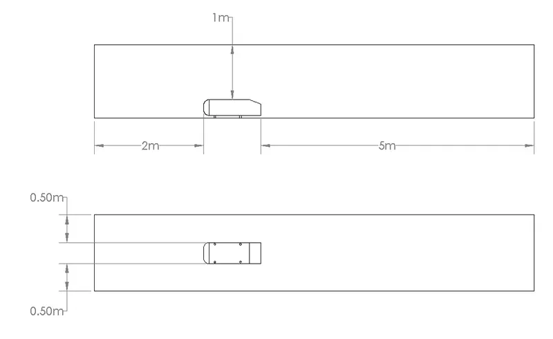
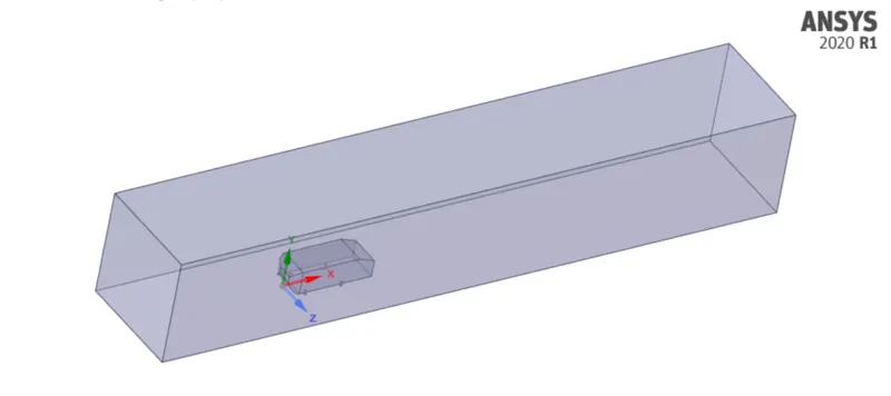
- Provide Enclosures to Ahmed body according to the given dimensions.
- Suppress Ahmed body.
- This completes the geometry step.
The Enclosure dimensions are
2.) Mesh -
- Start the mesh section
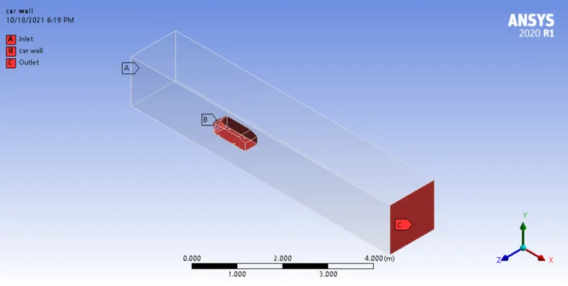
- Name the boundaries such as inlet, outlet and wall.
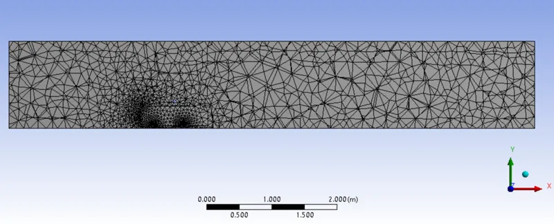
- Generate the mesh and then edit it with mesh size.
Generated mesh -
Named selection -
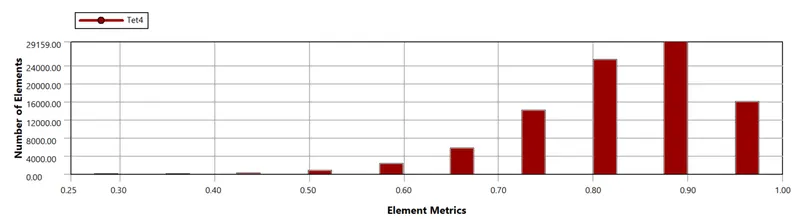
In order to see if the mesh we have generated is accurate or not, we'll check a quantity known as orthogonal mesh quality which tells us about the quality of our mesh.
3.) Solver -
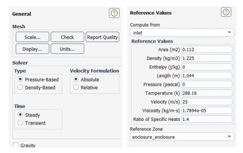
The first thing that we do is to select which type of solver we want to use that is either a steady-state solver or a transient state solver. We'll also have to give reference values for the calculation of drag and lift and we'll have to choose the laminar flow method only. All of which are shown below.
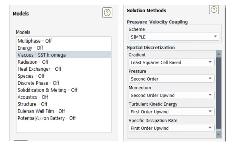
Now as we're done with setting up the solver, we can proceed to run the solver to get the desired result.
4.) Results -
Residual Plot -
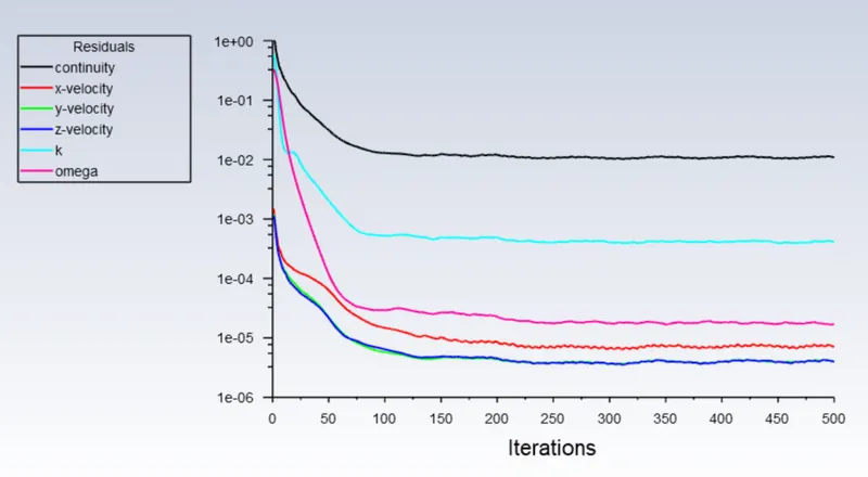
Drag Coefficient -
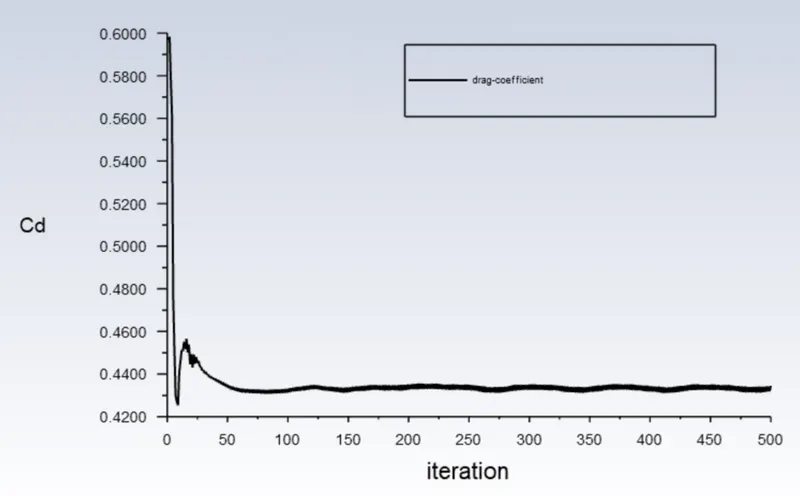
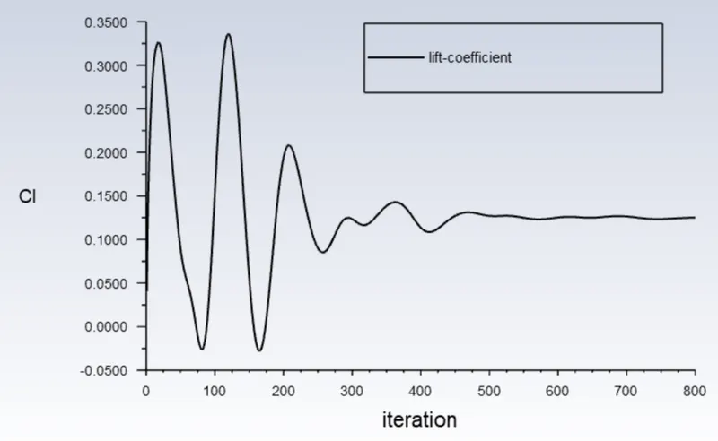
Lift Coefficient -
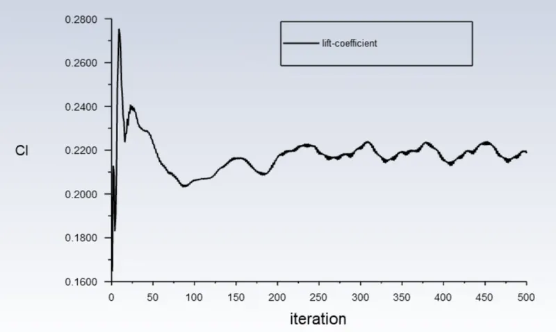
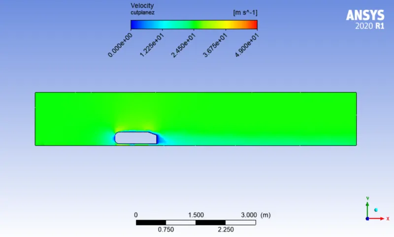
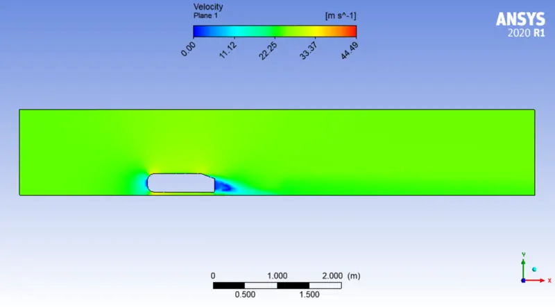
Velocity Contour -
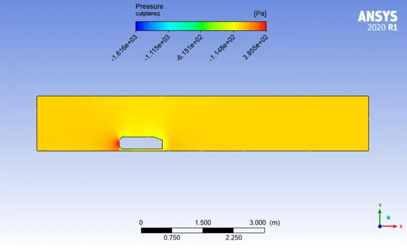
Pressure Contour -
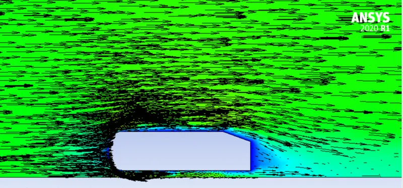
Vector Plot - Velocity
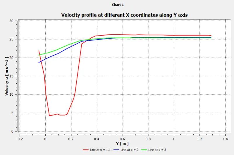
Velocity Data at (X,Y) - (1.1,2) , (2,2) , (3,3)
CASE 2 - Outer and Inner enclosure with fined mesh (Refined Y+ value)
1.) Geometry -
- Open the Geometry.
- Import the Ahmed Body.
- Split the body in half.
- Provide Enclosures to Ahmed body (Inner and outer) according to the given dimensions.
- Suppress Ahmed body.
- This completes the geometry step.
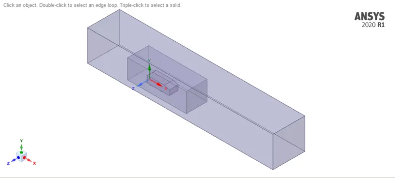
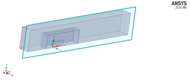
Now we cut our body along a cut plane as shown below. We're doing this in order to reduce the computational time by reducing the number of nodes. This is possible because our geometry is symmetric about the cut plane(XY plane) and we can use the symmetry boundary condition in order to get the result for the whole body.
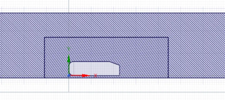
After both enclosures are created, we can check interference and avoid overlapping of meshing in the 2nd enclosure by applying check interference and deleting the overlap. This is automatically done by Spaceclaim when the interference option is selected inside prepare.
2.) Mesh -
- Start the mesh section
- Name the boundaries such as inlet, outlet and wall.
- Generate the mesh and then edit it with mesh size.
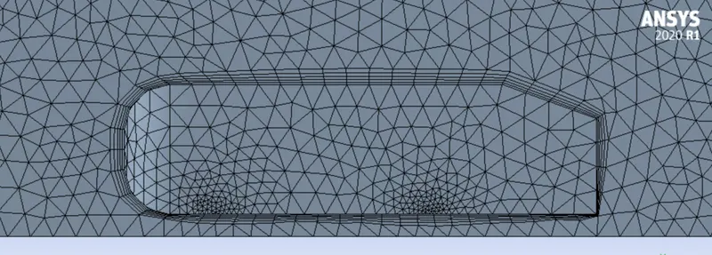
Generated mesh -
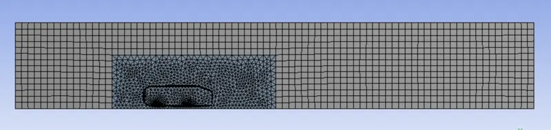
Element size for the first enclosure: 100mm.
Maximum size for the first enclosure: 100mm.
Element size for the second enclosure: 50mm.
Element size of pillars of Ahmed body: 5mm.
Number of elements: 91,327
Inflation layer: It is the process of adding layers to the boundary to cover the boundary layer thickness fully.
number of layers - 5
total thickness - 37.2mm with first layer thickness = 5mm.
`Y^+` = 349
Named selection -
Same as in the above cases.
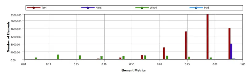
In order to see if the mesh we have generated is accurate or not, we'll check a quantity known as orthogonal mesh quality which tells us about the quality of our mesh.
3.) Solver -
The solver setting is the same as given in the above cases.
4.) Results -
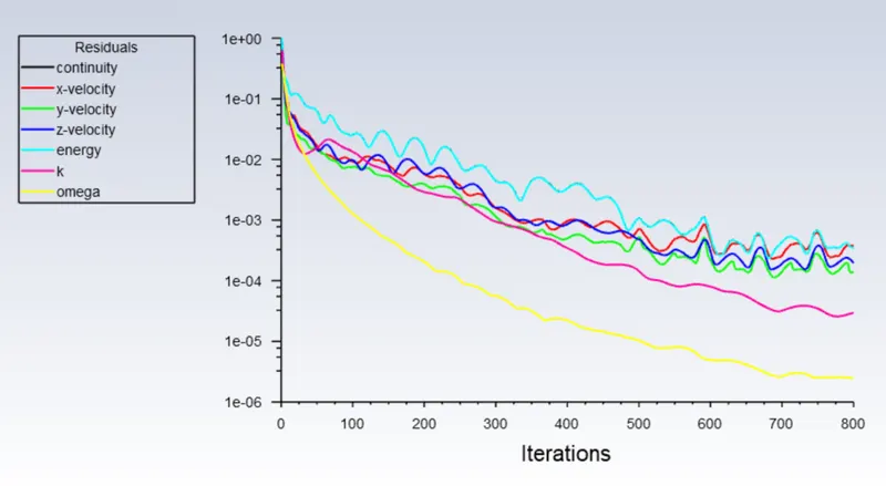
Residual Plot -
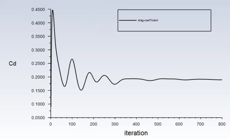
Drag Coefficient -
Lift Coefficient -
Velocity Contour -
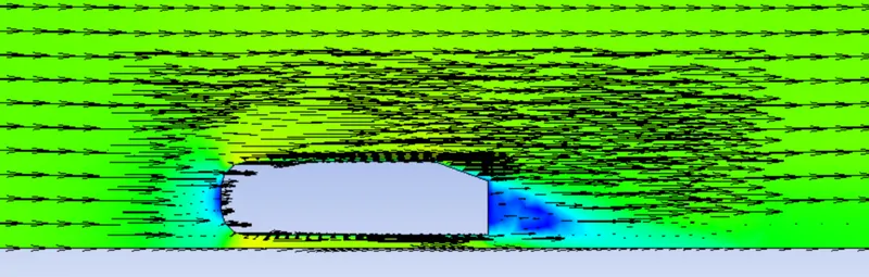
Vector Plot - Velocity
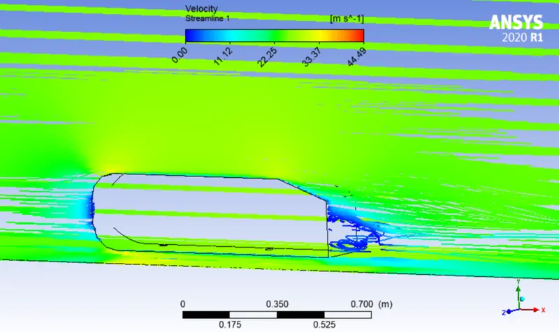
Velocity Streamline -
Pressure Contour -
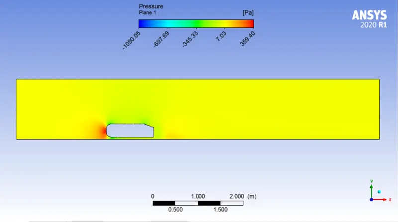
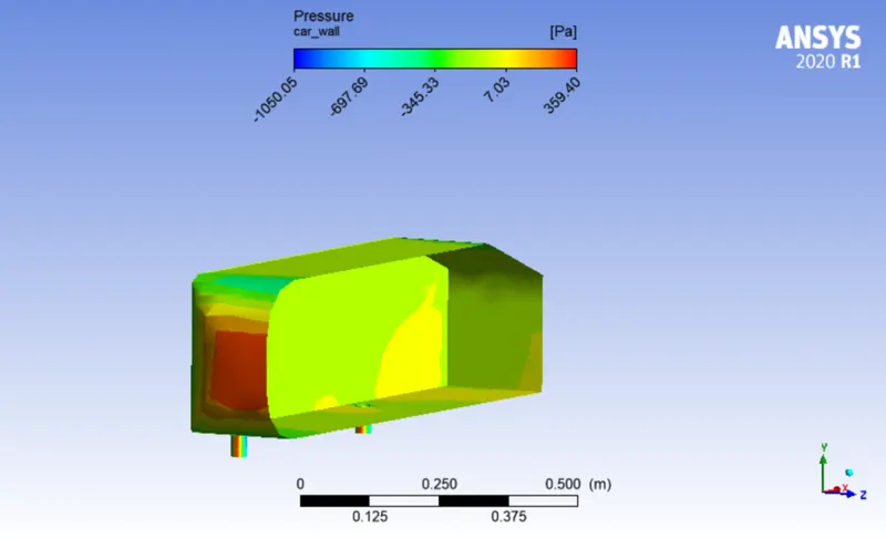
Pressure Contour at the Ahmed body-
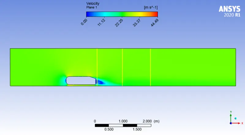
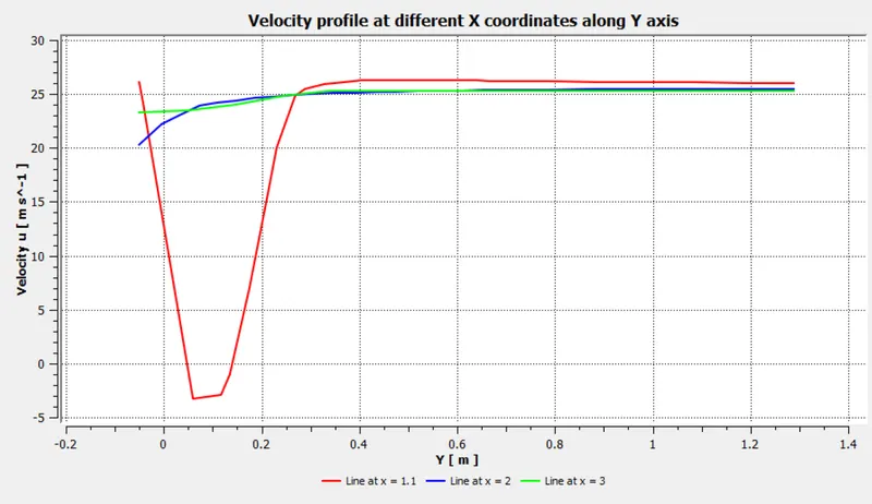
Velocity Data at (X,Y) - (1.1,2) , (2,2) , (3,3)
CASE 3 - More refined mesh (Refined Y+ value)
1.) Geometry -
Geometry is the same as in case 2.
2.) Mesh -
Generated mesh -
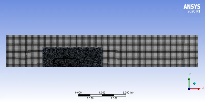
Element size for the first enclosure: 50mm.
Maximum size for the first enclosure: 100mm.
Element size for the second enclosure: 25mm.
Element size of pillars of Ahmed body: 5mm.
Number of elements: 5,35,038
Inflation layer: It is the process of adding layers to the boundary to cover the boundary layer thickness fully.
number of layers - 7
total thickness - 38.74mm with first layer thickness = 3mm.
`Y^+` = 209
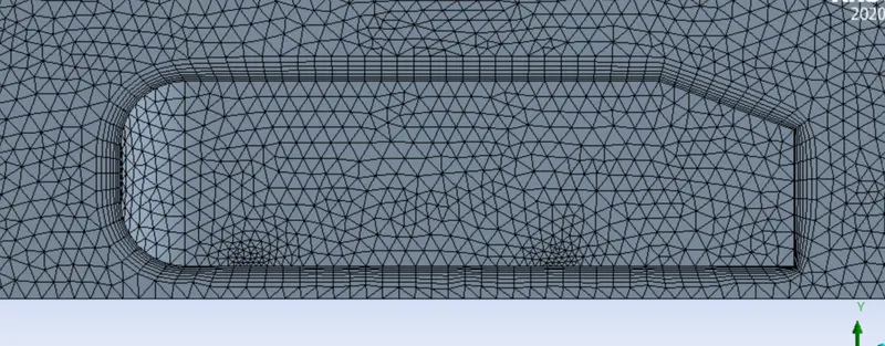
Named selection -
Same as in the above cases.
In order to see if the mesh we have generated is accurate or not, we'll check a quantity known as orthogonal mesh quality which tells us about the quality of our mesh.
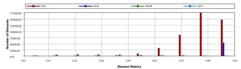
3.) Solver -
The solver setting is the same as given in the above cases.
4.) Results -
Residual Plot -
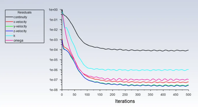
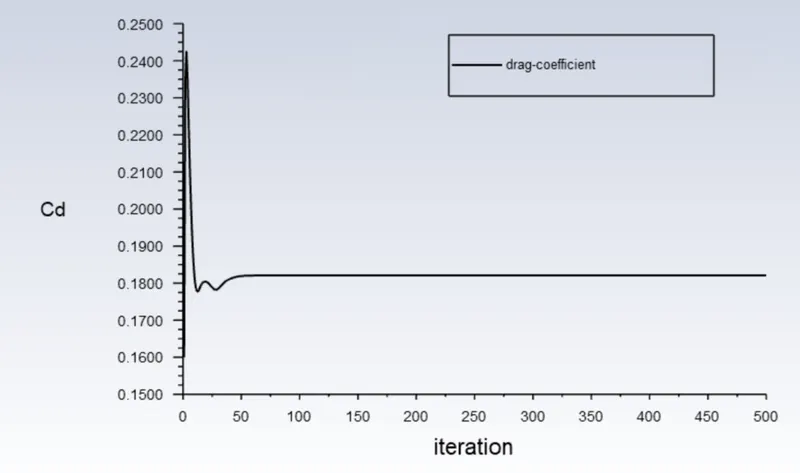
Drag Coefficient -
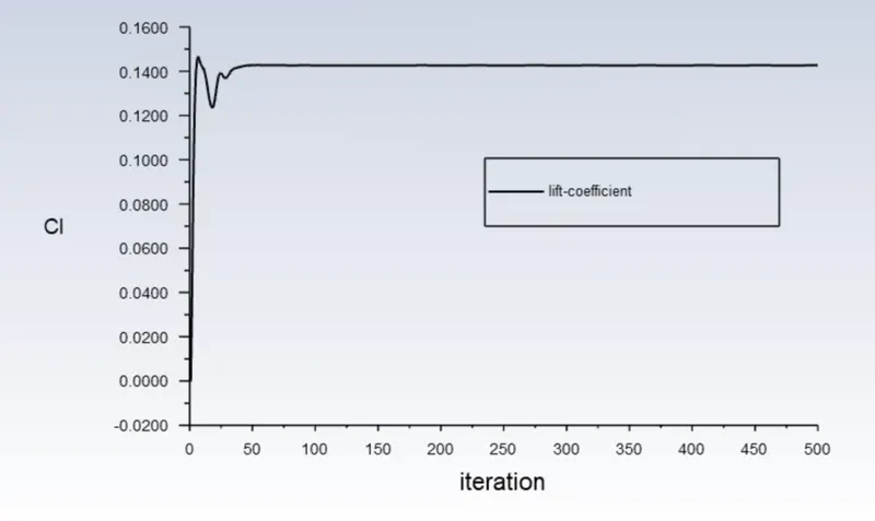
Lift Coefficient -
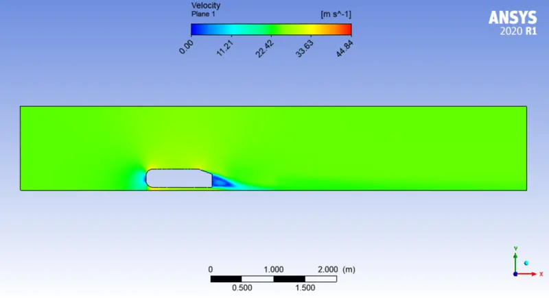
Velocity Contour -
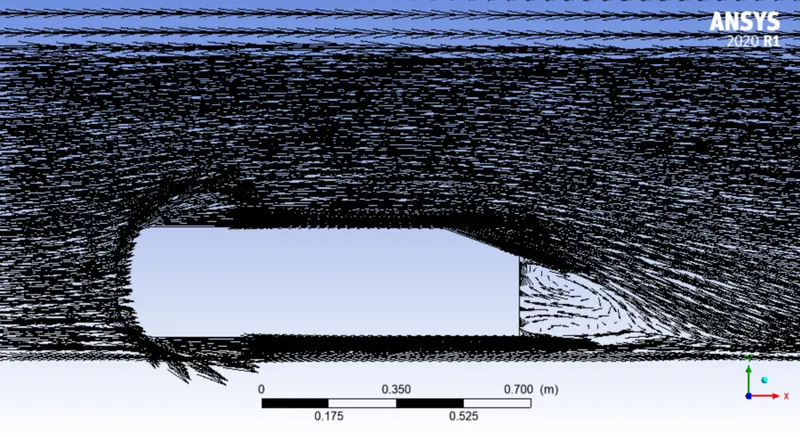
Vector Plot - Velocity
Velocity Streamline -
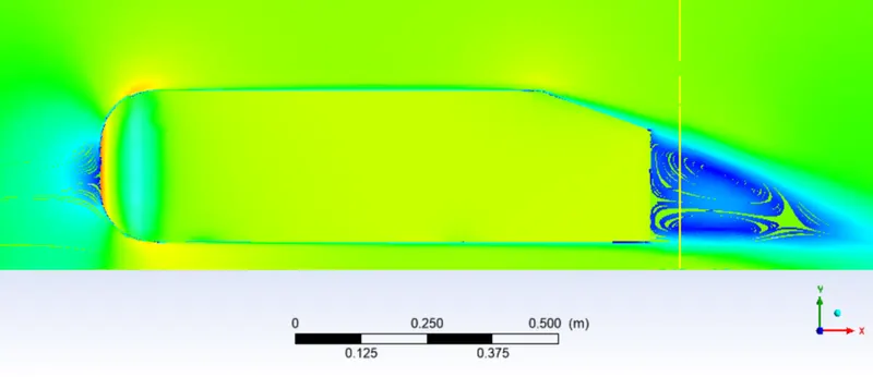
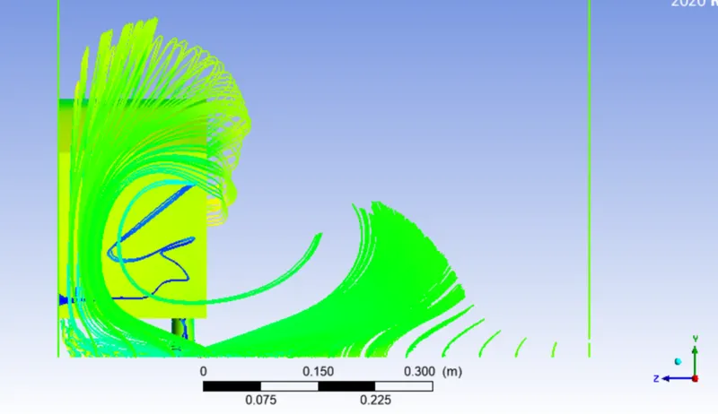
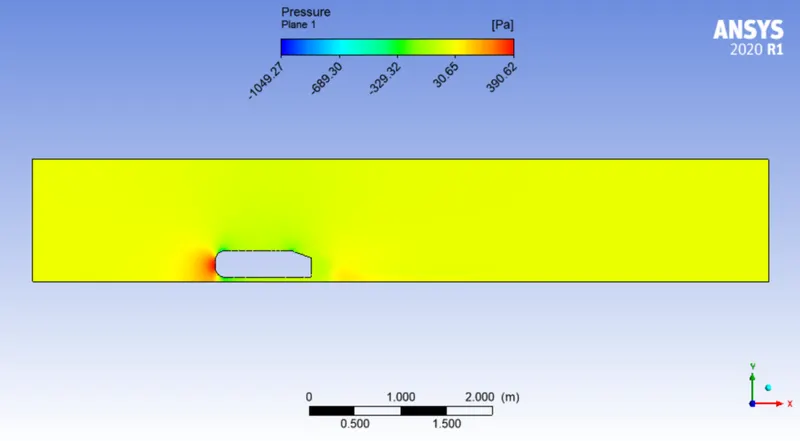
Pressure Contour -
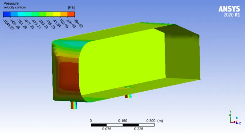
Pressure Contour at the Ahmed body-
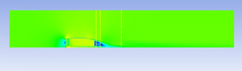
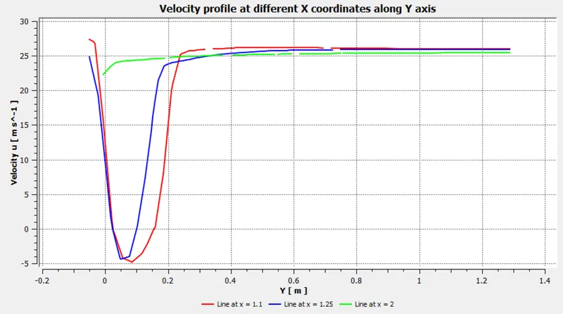
Velocity Data at (X,Y) - (1.1,2) , (1.25,2) , (2,3)
Grid Independence Test -
Comparison of all cases
It can be inferred that the imitation of the experimental result is obtained during the second refinement. Thus, the grid independence test saves a lot of computational time and convergence can be achieved by using smaller cell sizes for calculation.
Conclusion -
- It can be inferred that the grid independence test is performed to know the smaller cell size for convergence.
- Apart from mesh refinement, convergence depends on the Y+ value, inflation layer, it is advisable to use k – w (SST) as the turbulence model because it calculates the values well near the wall.
- As the setup is refined drag coefficient, lift coefficient decreases.
- Y+ plays an important role in determining the value of drag.
- The negative pressure in the wake region is primarily because there is no flow in that region. This can be further attributed to various factors such as separation and recirculation which is evident from the vector plot near the wake region.
- The point of separation occurs at the rear end of the vehicle; the separation occurs beyond this point where it can be observed that the flow recirculates and attaches it to the boundary layer.