External flow simulation over an Ahmed body.
AIM: TO PERFORM EXTERNAL FLOW SIMULATION OVER AHMED BODY.
OBJECTIVES:
Describe Ahmed's body and its importance.
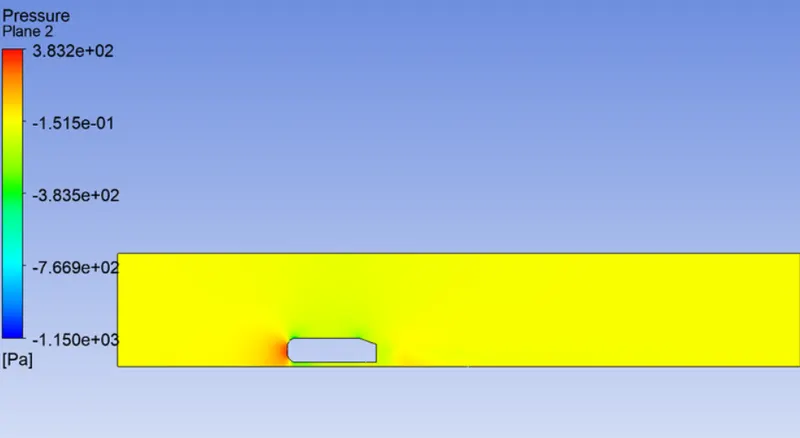
Explain the reason for the negative pressure in the wake region.
Explain the significance of the point of separation.
Expected Results:
1. Velocity and pressure contours.
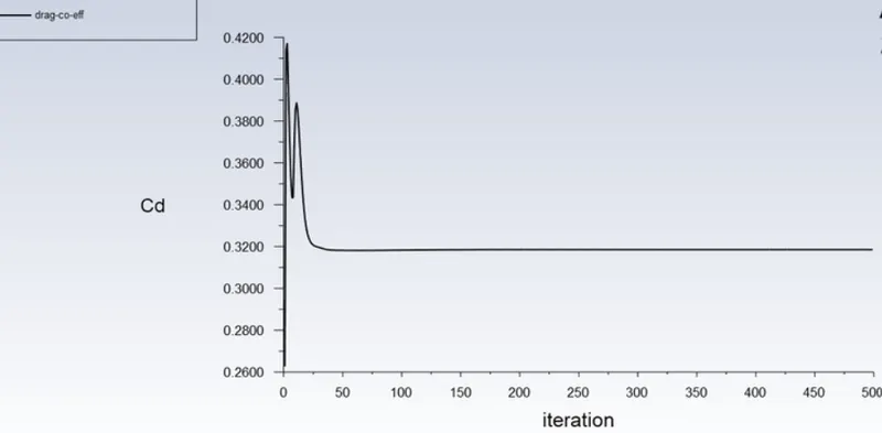
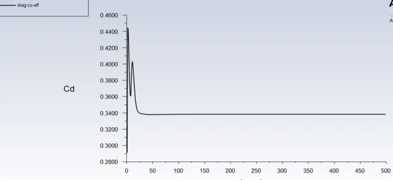
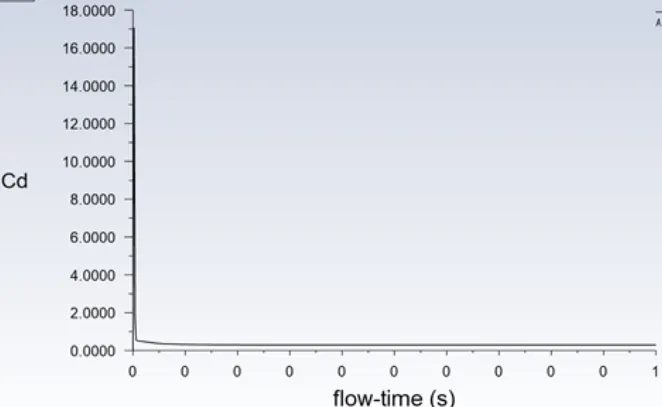
2. The drag coefficient plot for a refined case. ( For velocity of 25m/sec, the drag coefficient should be around 0.33).
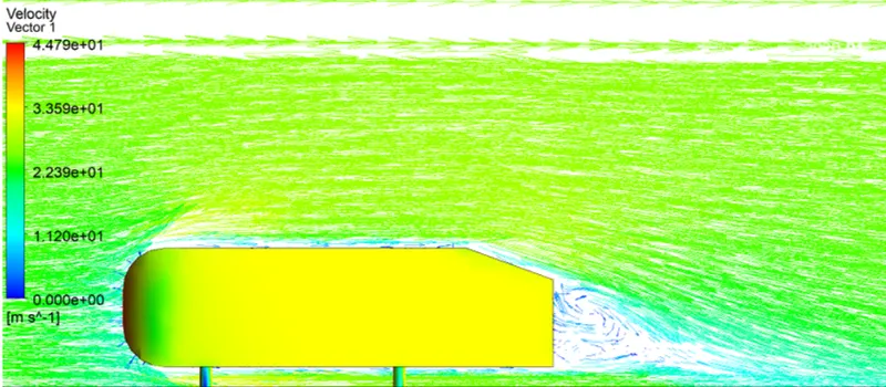
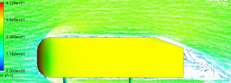
3. The vector plot clearly showing the wake region.
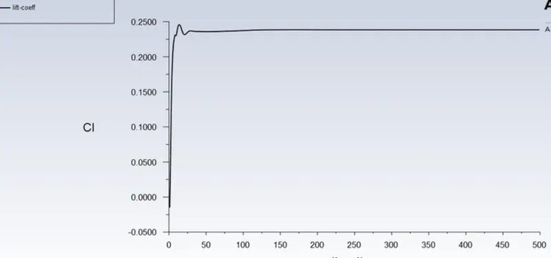
4. Perform the grid independence test and provide the values of drag and lift with each case.
INTRODUCTION:
Ahmed Body:
The Ahmed body is a generic car body (a simplified vehicle model). The airflow around the Ahmed body captures the essential flow features around an automobile and was first defined and characterized in the experimental work of Ahmed. Although it has a very simple shape, Ahmed body allows us to capture characteristic features that are relevant to bodies in the automobile industry.
This model is also used to describe the turbulent flow field around a car-like geometry. Once the numerical model is validated, it is used to design new models of the car.
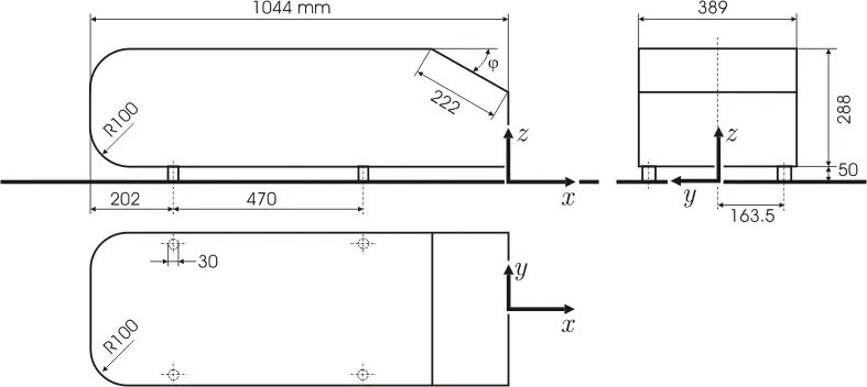
figure 1: Geometry of Ahmed Body.
DRAG COEFFICIENT
The drag coefficient quantifies the resistance of an object in a fluid environment. It is not an absolute constant for a body’s shape because it varies with the speed and direction of flow, object shape and size, and the density and viscosity of the fluid. The lower the drag coefficient of an object, the less aerodynamic or hydrodynamic drag occurs. In terms of a car, the lower the drag coefficient, the more efficient the car is. As well as affecting the top speed of a vehicle, the drag coefficient also affects the handling. Cars with a low drag coefficient are sought after, but decreasing the drag drastically can reduce the downforce and lead to a loss in road traction and a higher chance of car accidents.
There are two types of drag forces that are applied to a object:
1) Pressure Drag: Pressure drag is caused by adverse pressure gradient.
2) Skinfricition Drag: Caused by sheer stress resistance due to the law of wall and viscous nature of fluid.
`underset(d)(C)=2*(Fd)/(rho*V^2*A`
where Cd=Drag coefficient
Fd=Drag force
A=Area
V=Velocity
NEGATIVE PRESSURE IN WAKE REGION
When the air moving over the vehicle is separated at the rear end, it leaves a large low-pressure turbulent region behind the vehicle known as the wake. This wake contributes to the formation of pressure drag, which eventually reduces the vehicle performance.
The region of recirculating flow immediately behind a moving or stationary blunt body, caused by viscosity, which may be accompanied by flow separation and turbulence flow, or the wave pattern on the water surface downstream of an object in a flow, or produced by a moving object (e.g. a ship), caused by density differences of the fluids above and below the free surface and gravity. When the vehicle is moving at a certain velocity, the viscous effects in the fluid are restricted to a thin layer called the boundary layer. Outside the boundary layer is the inviscid flow. This fluid flow imposes pressure force on the boundary layer.
When the air reaches the rear part of the vehicle, the fluid gets detached. Within the boundary layer, the movement of the fluid is totally governed by the viscous effects of the fluid. The Reynolds number is dependent on the characteristic length of the vehicle, the kinematic viscosity and the speed of the vehicle. The fluid moving around the vehicle is dependent on the shape of the vehicle and the Reynolds number. There is another important phenomenon, which affects the flow of the car and the performance of the vehicle. This phenomenon is commonly known as the ‘Wake’ of the vehicle. When the air moving over the vehicle is separated at the rear end, it leaves a large low-pressure turbulent region behind the vehicle known as the wake. This wake contributes to the formation of pressure drag, which eventually reduces the vehicle performance.
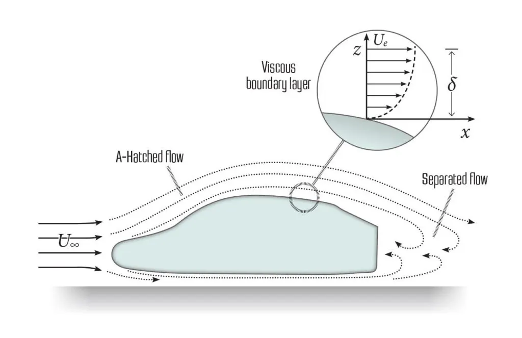
Figure 2: Wake region
POINT OF SEPARATION
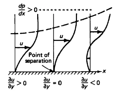
Figure 3: Flow Separation
Separation of flow is said to occur when the direction of the flow velocity near the surface is opposed to the direction of the free stream velocity, which means` (du)/(dy) ≤ 0`. Such a situation arises when there is a negative pressure gradient near the wall (Refer Fig.3). An example is a subsonic diffuser or rear portion of the car.
In the direction of flow the pressure increases which causes decreases in velocity and creates conditions for separation to occur. It is important to note that, the skin-friction coefficient reaches the value zero. At this point, the wall shear stress vanishes is called the separation point.
Reverse flow takes place beyond the point of separation. Due to reverse flow, irregular eddies are formed and a lot of energy is dissipated. This region is called "Wake". The pressure distribution in the wake is quite different from that on the remaining boundary and this gives rise to an additional drag force on the body. Wake also leads to lateral vibration to the object which may be harmful. Also, a large amount of K.E. is lost.
In the turbulent boundary layer, some of the energy is dissipated in friction, slowing airflow velocity, resulting in a pressure increase. If the increase in pressure is gradual, the process of turbulent mixing will cause a transfer of energy from the fast-moving eddies to slower ones in the turbulent boundary layer. If the rate of change in pressure is too great, for example in sharp corners, the mixing process will be too slow to push the slower air molecules moving. When this happens, the boundary layer flow stops following the contours of the surface, resulting in separation. Air particles downstream of the separation region will then move towards the lower pressure region in the reverse direction to the main flow, the separation region will reattach.
In the region between separation and reattachment points, airflow is circulating and this is called the „separation bubble Separation will normally occur if the resultant flow encounters a sharp edge and that is why it is always important for ground vehicles to have smoothly rounded edges everywhere.
Steps to Prepare Geometry and Run the Simulation
1. Model is imported into Spaceclaim window as shown in figure 4.
a. Drawn the bigger & smaller enclosure(for mesh refinement near the boundary of car-wall that is where we need more accurate results) for wind-tunnel simulation of Ahmed body.
b. Check the interference region.
c. Use of options shared topology for transfer information to each other.
2. Open the Mesh window, the name given to domain-like(Inlet, outlet, symmetry, bottom wall, car wall).
a. Give element size & body sizing to bigger, small enclosure, car wall, car stand for coarse to finer mesh.
b. Addition of inflation layer to get accurate the solution near the wall.
3. Open the Setup & solution window.
a. Choose the Turbulence model like K-epsilon & k-omega model & also turn on energy eq.
b. Give the boundary condition like inlet velocity 25m/s, outlet zero gauge pressure.
c. Prepare report Coefficient Drag, lift. Check the Y+ criteria.
4. Open Result window.
a. Plot the velocity & Pressure contour.
b. Plot the velocity vector plot.
5. Analysis of Coefficient Drag & lift, Wake region, Pressure distribution.
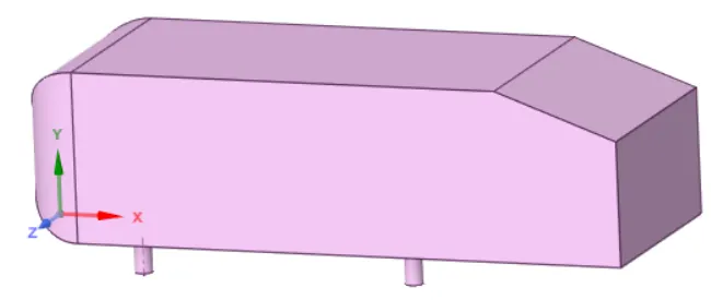
Figure 4:Ahmed Body Model
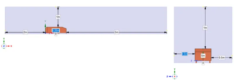
Figure 5. The enclosure is prepared as a wind tunnel.
The best practice for symmetric objects and problems is that we can do analysis on 1/2 geometry and expect symmetric results for the other part. By this, we can save computation time. This reduces the number of cell counts.
We can use the split body command to delete half body about the symmetric plane in our case it's the XY plane.
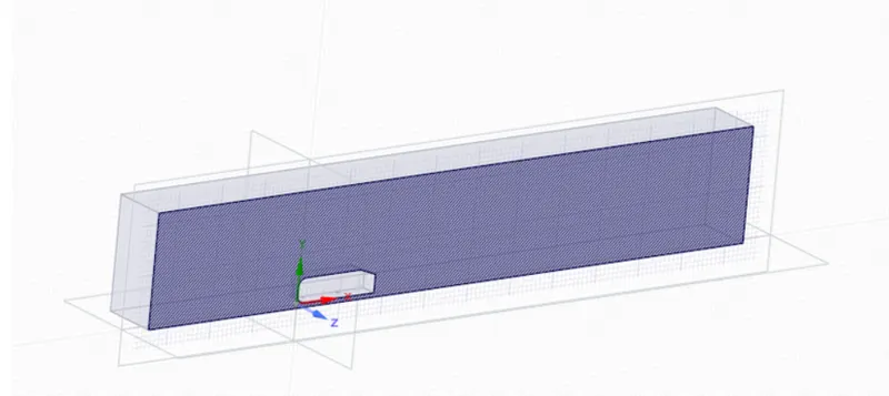
Figure 6. Plane XY is used for splitting the geometry.
Named Selections are given as
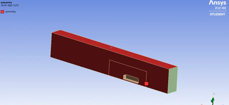
Figure 7. Symmetry for all walls of enclosure
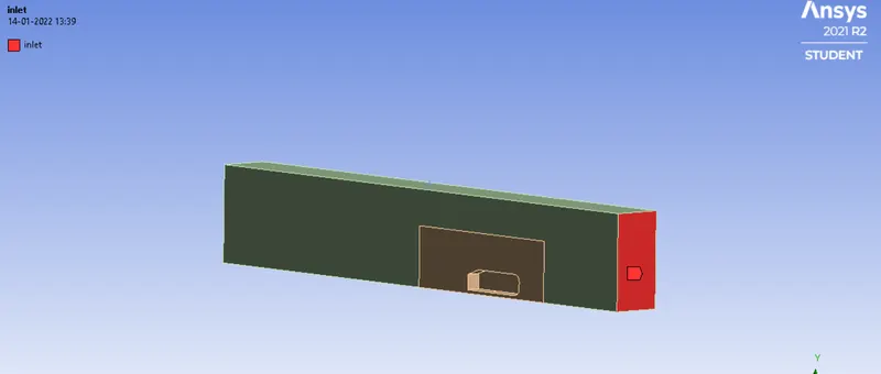
Figure 8. Inlet
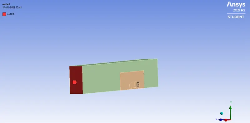
Figure 9. Outlet
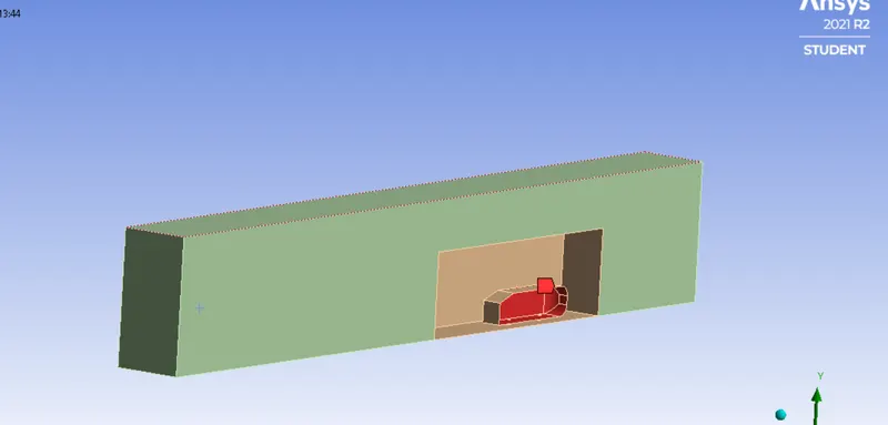
Figure 10. Car-wall
Meshing
Method
Outside the box, the hexahedral mesh is used. The mesh is of the highest quality and gives higher accuracy.
Multizone method: It is used to create hexahedral meshes wherever possible and for other regions where different mesh types are used it will connect it properly.
Sizing: It is defined as increasing the number of elements by decreasing the element size.
Element size for the first enclosure:100mm or 0.1
Maximum size for the first enclosure: 100mm or 0.1mm
Element size for the second enclosure: 50mm
Element size of pillars of Ahmed body: 5mm
Number of elements : 1,92,628
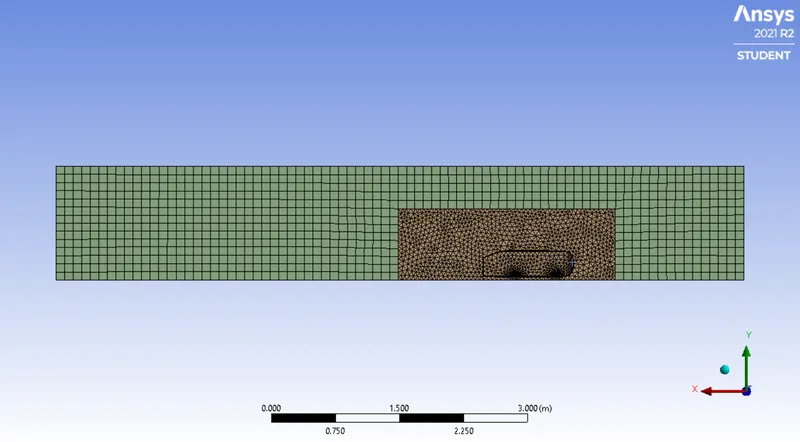
Figure 11. Hexahedral mesh in outside enclosure and tetrahedral mesh (more refined inside enclosure).
Estimation of first cell thickness (y+) :
a) First we need to calculate the reynold's number for flow problem.
`Re=(rhoVL)/mu`
here `rho`=density=1.225`(kg)/m^3`
`V`=velocity=25`m/s`
`L`=Length of object=1.04m
`mu`=dynamic viscosity=`0.000017894(kg)/(m*s)`
So Re = 1779926.2322
b) Skin Friction Coefficient for external flows is,
`Cf=0.058*(Re)^-0.2`
Cf = 0.0032609
c)Wall shear stress ,
`tau=(1/2)*Cf*rho*U^2`
tau = 0.5*0.0032609*1.225*25*25 = 1.248 kg /m-s^2
d)Shear Velocity
`U_tau = sqrt{frac{tau_w}{rho}}`
Shear velocity, Ut = 1.009 m/s
e)Now finally to calculate first cell thickness, △y
y+=1, (Since `k-omega` is the turbulence model due to low reynolds number) First cell thickness,
`△y=((y+)*mu)/(rho*U_tau)
=1.426e-5
f) So total thickness of inflation layers with 6 layers and cell height=1.426e-5 is given by sum of Geometric Progression
`S_n=a.(1-r^n)/(1-r)`
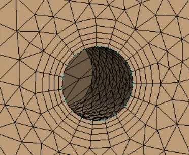
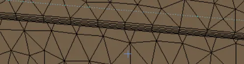
Figure 12. Refinement around pillars and inflation layers for capturing near-wall drag.
SOLVER SETUP:
For the solver setup, a pressure-based solver is used rather than a density-based solver by calculating the Reynolds number. The fluid which is used throughout the simulation is Air. The inlet boundary condition is considered as velocity inlet of 25 m/s and the outlet boundary condition is considered as pressure outlet (atmospheric pressure). It is necessary to define the car wall as a boundary of the wall with no-slip conditions to evaluate the drag coefficient. For reference values, the frontal area of the Ahmed body 0.131482m2 is provided as area and the length is given as 1.044 m. The SIMPLE algorithm is chosen for the pressure-velocity coupling. For solution animation, a reference frame or plane is required on which the results are displayed. This can be done by using the location option in which a plane is created for reference.
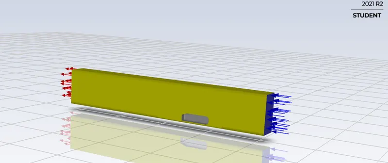
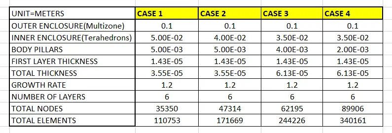
Figure 13: Meshing is set up for different cases
CASE 1
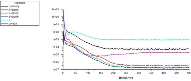
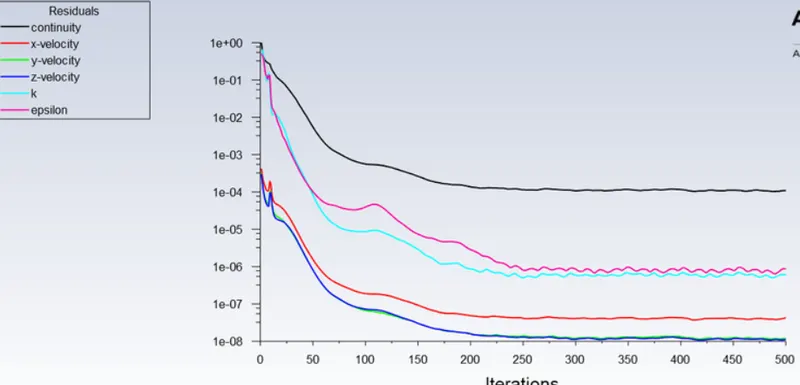
Figure 14. Residuals
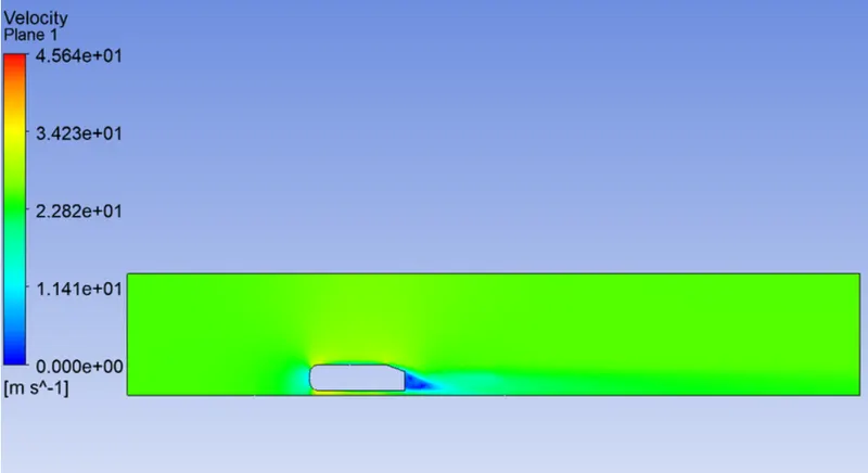
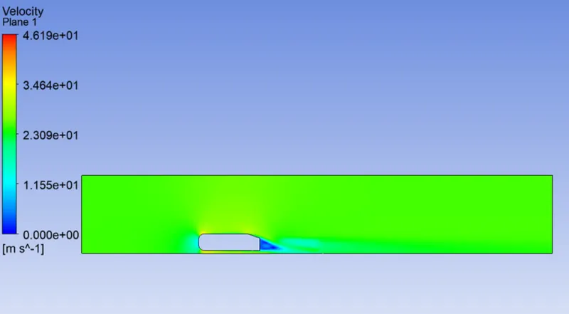
Figure 15. velocity contour
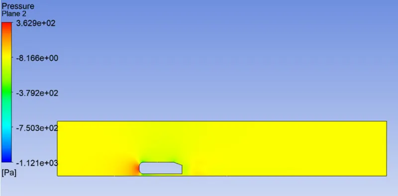
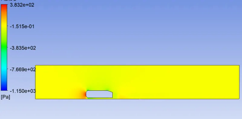
Figure 16. Pressure Contour
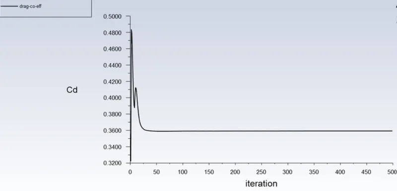
Figure 17. Drag coefficient plot
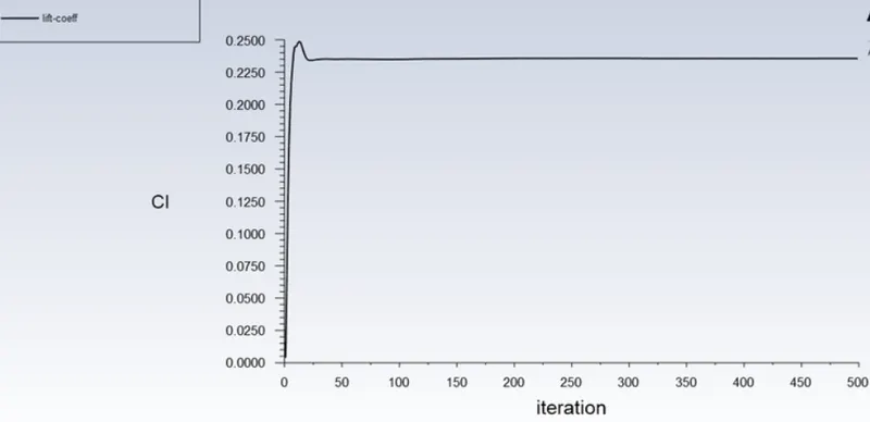
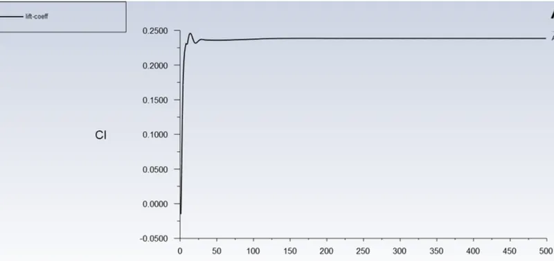
Figure 18. Lift plot
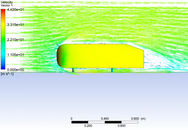
Figure 19. Vector Plot
Case 2
CASE 3
CASE 4
In case 4 Cd values started to decrease, thus case 3 is the most accurate simulation.