Week 3 - External flow simulation over an Ahmed body.
Objective: To perform the grid independency test on Ahmed body.
Expected result:
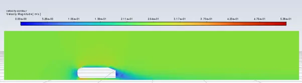
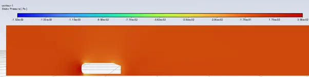
- Velocity and pressure contour.
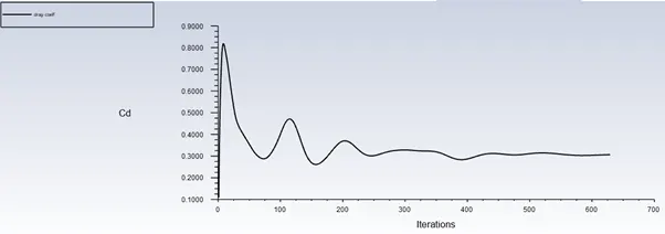
- The drag coefficient plot for refined case.
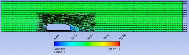
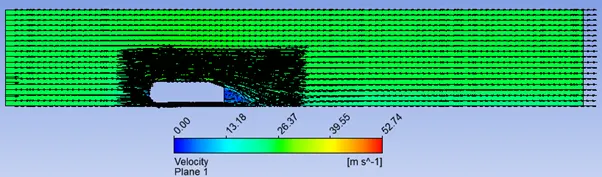
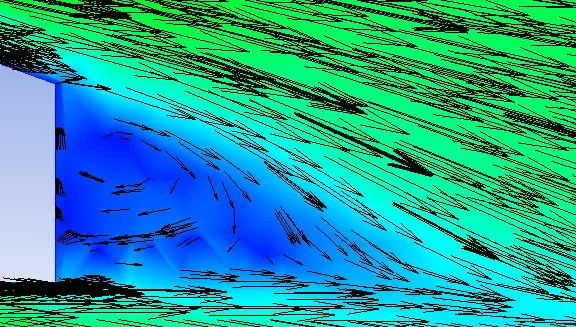
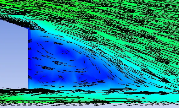
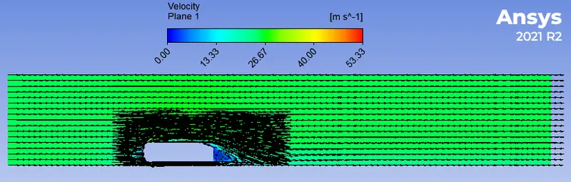
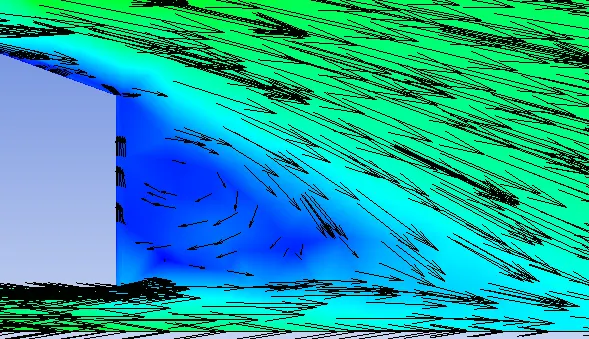
- The vector plot showing the wake region.
- Provide drag and lift coefficient value for each case.
Given data
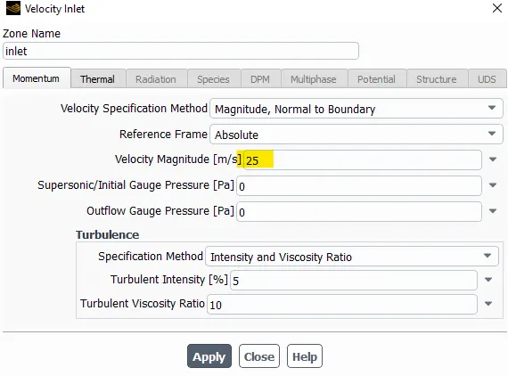
Flow velocity of air = 25 m/sec.
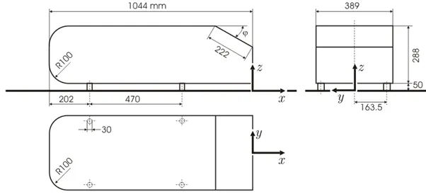
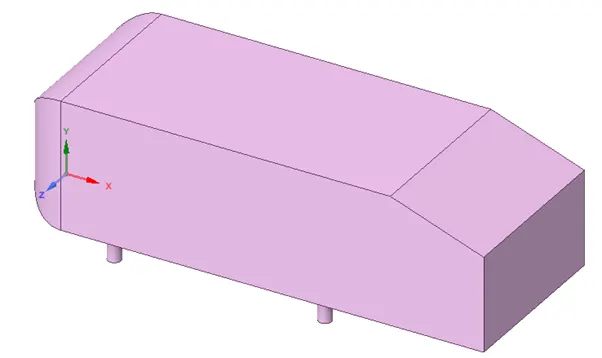
The geometry of the Ahmed body along with all dimensions is as given below in the figure.
Theory
The Ahmed body is a generic car body (a simplified vehicle model). The air flow around the Ahmed body captures the essential flow features around an automobile like wake forces, drag forces etc. and was first defined and characterized in 1984 by Ahmed et. al. the Ahmed body is designed to have smooth-edged front end with a flat roof and a flat bottom section and an angle back slant which basically acts as the rear window of a car end ending with a vertical base. The back slant angle which is commonly designed as $ is very critical to the flow patterns which are fashioned at the near wake reason and subsequently has an impact on the aerodynamic forces which act on the body. Car companies makes numerous attempts to develop modified designs to effectively reduce the aerodynamic drag force which occurs at the rear end without putting any constraints in the stability, comfort and safety of the passenger. The aerodynamic drag of road automobiles is firmly connected to the vehicles with downstream flow. The separation zone size and the drag force directly rest mainly on the position of flow separation over the Ahmed body. Subsequently, comprehensive facts regarding the wake flow characteristics and its connection with the geometry of body is essential for a successful design of upcoming future cars. The application of computational fluid dynamics in in determining fluid flow pattern has been observed to be very common among researches in the present days. CFD Modelling in determining flow line of fluid around the Ahmed body has been utilized since the early `21^(st)` century. In many open literatures the CFD application in determining air flow pattern and the changes in flow motion with altering geometry of the body have been found. Certain modifications in the and body aids researches and designers to determine the effect of modification on the resultant drag and lift force which can be calculated using CFD modelling. Purpose of automotive is reduction of drag, decreasing noise emission, increasing fuel economy and eliminating unnecessary lift force and other origin of aerodynamic unsteadiness which rises at high speed. The conventional and reference model has been considered as the standard model in this research work for carrying out numerical simulations for researching on the aerodynamic parameters the Ahmed body has a like featured like a general car and is broadly utilized for authentication of new quotes in the automobile industry. This simple geometric model has a length of 1.044 m height of 0.288m and a width of 0.389 m. It consists of cylindrical legs of 0.5 m radius attached to the bottom most part of the body. The real most surface has an inclination of 25 degree. Ahmedabad characterizes the simplified geometry of a ground vehicle as a bluff body type. Its geometry is adequate enough for precise flow simulation and returns few vital practical features relevant to cars. This model aids engineers and designers to generate turbulent flow field surrounding the simple car model by the use of K-epsilon model. In spite of neglecting quite a few numbers of features of a real car like rough underside rotating wheels, surface projection etc. Ahmed body generates the crucial feature of flow pattern around a car for instance flow impinge-mentation and the displacement around the nose, relative uniform flow of air around the middle portion and flow separation along with the wake generation at the rear. Since the Ahmed body is easy to model, it can be a place is utilized for researching various properties like turbulence, drag coefficient, wake reason, lift forces, velocity magnitude at various regions of the car. Magnitude of pressure around the car which helps in in determining what will be resistance, fuel efficiency etc. Of the car thereby providing designers a clear Idea on which reason needs to be optimized for better effectiveness. The main objective of this study being stimulation of turbulent flow within the wind tunnel and around the Ahmed body to capture the flow pattern at the rear and wake region. Are local refinement of mess inside the concerned body is done with necessary body and face sizing of the parts of the body to generate well defined plots for pressure and velocity contours and its grid dependency test is the primary focus of this project.
Negative pressure in the wake region and point of separation
Wake region:
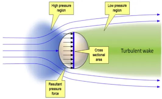
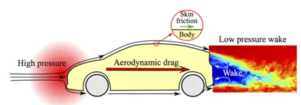
Consider a fluid particle flows within the boundary layer around the circular cylinder. From pressure distribution measured, the pressure is maximum at the stagnation point and gradually decreases along the front half of the cylinder. the flow stays attached on this favorable pressure reason as expected. However, the pressure starts to increase in the rear half of the cylinder and the particles now experiences as adverse pressure gradient. consequently, the flow separates from the surface and creating a highly turbulent region behind the cylinder called ‘Wake’. the pressure inside the wake region remaining low as the flow separates and a net pressure force(pressure drag) is produced.
Flow separation:
The presence of the fluid viscosity slows down the fluid particles very close to the solid surface and forms a thin slow moving fluid layer called a boundary layer. The flow velocity is zero at the surface to satisfied the no slip boundary condition. Inside the boundary layer, flow momentum is quite low since it experiences a strong viscous flow resistance. Therefore, the boundary layer flow is sensitive to the external pressure gradient (As the form of a pressure force acting upon fluid particles). if the pressure decreases in the direction of the flow, the pressure gradient is said to be favorable. In this case, the pressure force can assist the fluid movement and there is no flow retardation. However, if the pressure is increasing in the direction of the flow. an adverse pressure gradient condition as so it is called exist. In addition to the presence of a strong viscous force the fluid particles now have to move against the increasing pressure force. Therefore, the fluid particles could be stopped or reversed, causing the neighboring particles to move away from the surface. this phenomenon is called the boundary layer separation.
The pressure gradient is one of the factors that influence the flow immensely. As discussed above, a negative pressure gradient is termed a favorable pressure gradient. such a gradient enables the flow. a positive pressure gradient has the opposite effect and is termed the adverse pressure gradient. Fluid might find it difficult to negotiate an adverse pressure gradient. Sometimes, we say the fluid has to climb the pressure hill. One of the sewer effects on an adverse pressure gradient is to separate the flow.
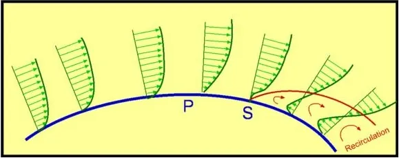
Consider flow past a curved surface as shown in figure. the geometry of the surface is such that we have a favorable gradient in the pressure to start with and up to a point P. the negative pressure gradient will counteract the retarding effect of the shear stress (which is due to viscosity) in the boundary layer. For geometry considered we have an adverse pressure gradient downstream of P.
Now the adverse pressure gradient begins to retard. this effect is felt more strongly in the regions close to the wall where the momentum is lower than in the regions near the free stream. as indicated in the figure. the velocity near the wall reduces and the boundary layer thickens. continuous retardation of flow brings the wall shear stress at the point S on the wall to zero. from this point onwards the shear stress becomes negative and the flow reverses and a region of circulating flow develops. We see that the flow no longer follows the contour of the body. we say that the flow has separated. this point S where the shear stress is zero is called the separation point.
Case setup
Geometry
- Import Ahmed body geometry in the SpaceClaim.
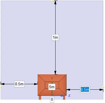
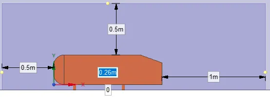
- Prepare an Enclosure for the Ahmed body
Side view

Front view
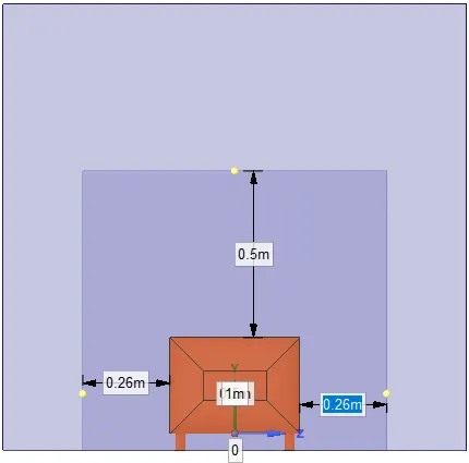
- Add another Enclosure of smaller dimensions.
Side view
Front view
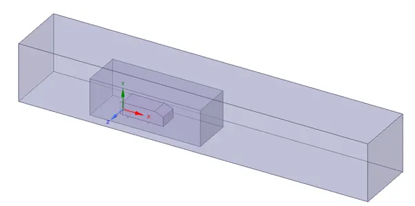
Final geometry after adding Enclosures is shown below:
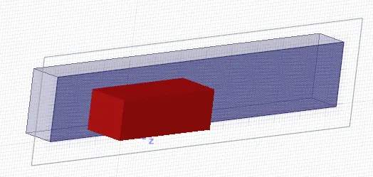
- Add a plane and view in section mode for the interference.
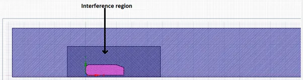
- In prepare section click on interference it will show interference region.
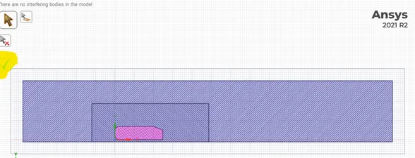
- Press on green tick and I will resolve the interference problem.
Resolved interference
- Suppress the Ahmed body for physics.
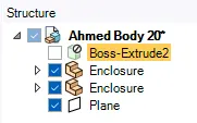
- Close SpaceClaim.
Meshing
- Open meshing interface and click on generate mesh at default values.
Baseline mesh is show below:
Side view

Bottom surface
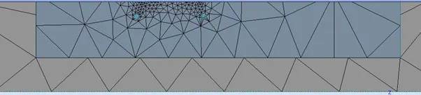
- Now insert a meshing method and for method use multizone. When we will use multizone it will automatically use hexahedral mesh where ever possible.

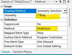
- Select the outer box and apply in geometry
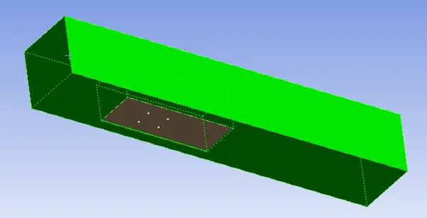
Generated mesh for outer box is shown below:

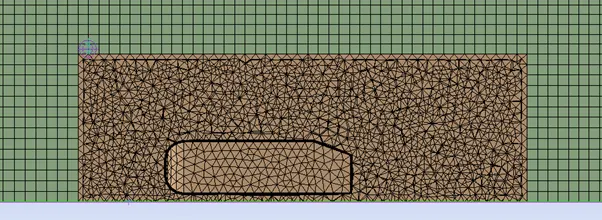
- Now insert sizing and select inner box as geometry and element size as per requirement and generate mesh.
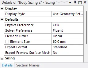
Generated mesh is shown below:
- Insert sizing and select 4 cylindrical stands of the body for the geometry and apply and set element size as per requirement.
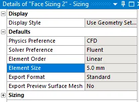
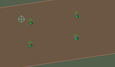
Generated mesh is shown below:
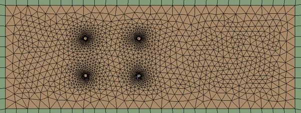
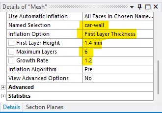
- Add inflation layer to the car-body surface and select inflation option as ‘first layer thickness.
- First layer hight as calculated from Y_p.
- Maximum layers = 6
- Growth rate = 1.2
Generated mesh is shown below:
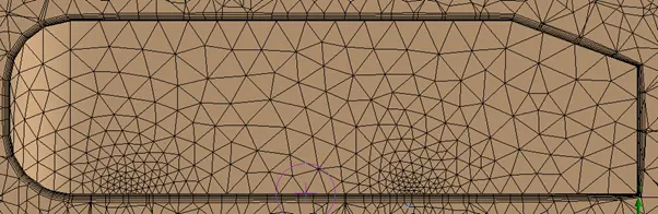
Inflation layers:

- close meshing
Setup
- open fluent setup and perform mesh check to ensure mesh generated is free from errors.
Set Reference values
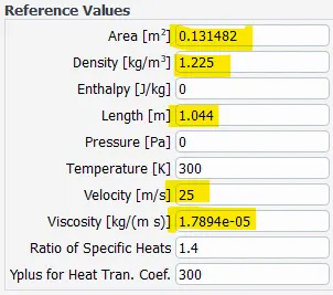
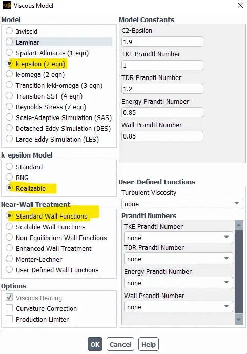
- change viscous model to realizable k-epsilon model and chose standard wall function.
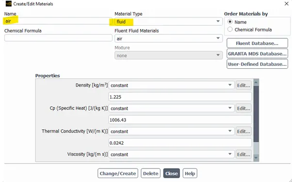
- Add material type as fluid and material air.
- Change boundary conditions:
- Car wall = wall
- Outlet = pressure outlet
- Symmetry = symmetry
- Inlet = velocity
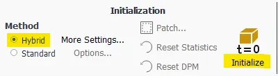
- Now perform hybrid initialization.
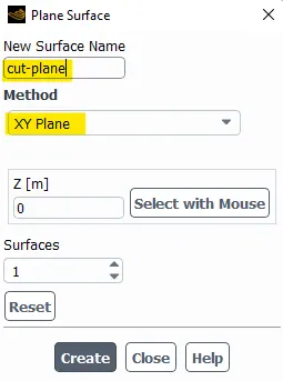
- Create a XY cut-plane.
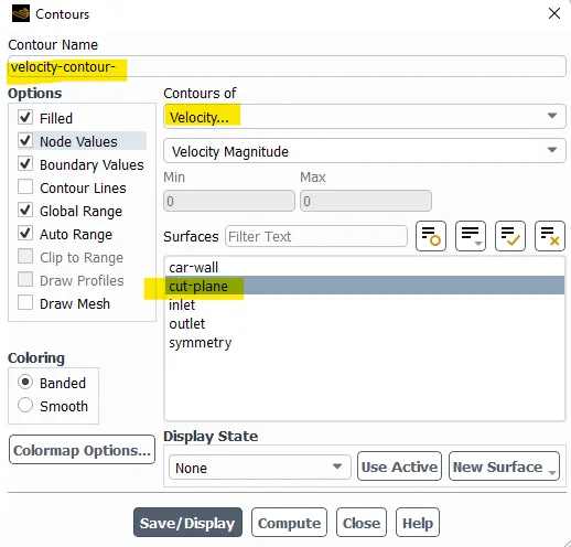
- Create a velocity contour at cut-plane.
- Similarly create a pressure contour.
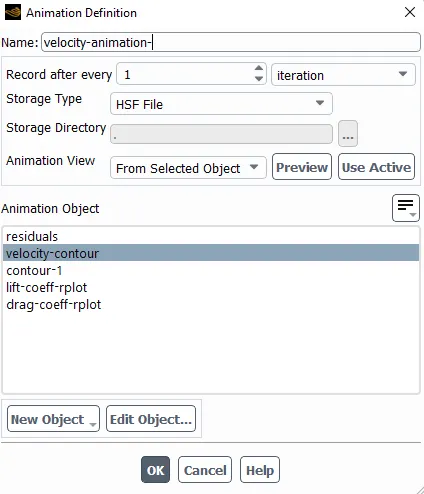
- Create animation for velocity contour.
- Create a definition for drag coefficient.
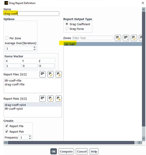
- Similarly create definition for lift coefficient.
- Run calculation
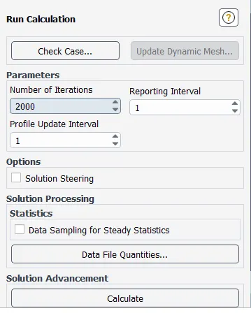
Output from the simulation
Case – 1
For bigger Enclosure
Mesh element size = 100mm
Maximum size = 100mm
Inflation (car wall) no. of layers = 6
Growth rate = 1.2
Inflation option = first layer thickness
First layer thickness = 1.4mm
For smaller Enclosure
Body sizing
Element size = 100mm
Face sizing bottom leg
Element size = 5mm
No. of nodes = 42504
No. of elements = 97818
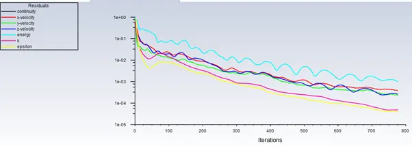
Residuals
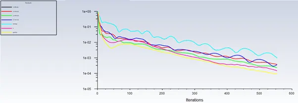
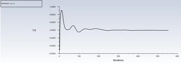
Coefficient of drag
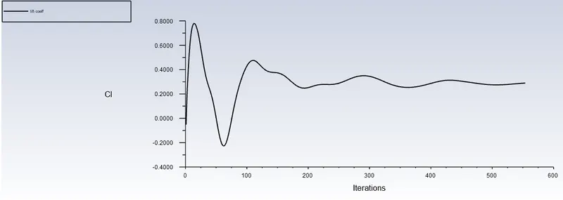
Coefficient of lift
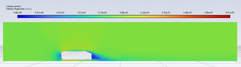
Velocity contour
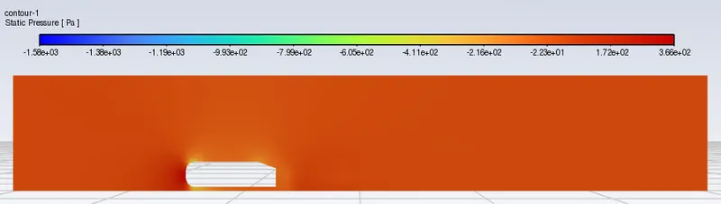
Pressure contour
Vector plot
Case – 2
For bigger Enclosure
Mesh element size = 80mm
Maximum size = 100mm
Inflation (car wall) no. of layers = 6
Growth rate = 1.2
Inflation option = first layer thickness
First layer thickness = 1.4mm
For smaller Enclosure
Body sizing
Element size = 60mm
Face sizing bottom leg
Element size = 5mm
No. of nodes = 66071
No. of elements = 156569
Residuals
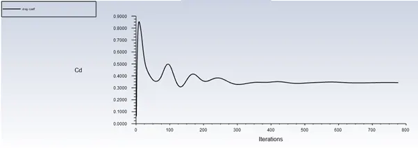
Coefficient of drag
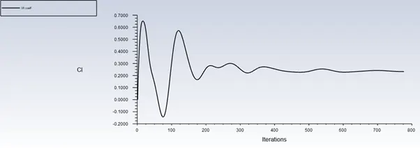
Coefficient of lift
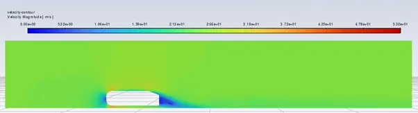
Velocity contour
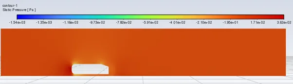
Pressure contour
Vector plot
Wake region
Case – 3
For bigger Enclosure
Mesh element size = 60mm
Maximum size = 100mm
Inflation (car wall) no. of layers = 6
Growth rate = 1.2
Inflation option = first layer thickness
First layer thickness = 1.4mm
For smaller Enclosure
Body sizing
Element size = 50mm
Face sizing bottom leg
Element size = 5mm
No. of nodes = 113185
No. of elements = 242304
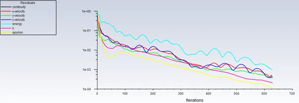
Residuals
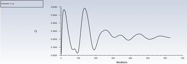
Coefficient of drag
Coefficient of lift
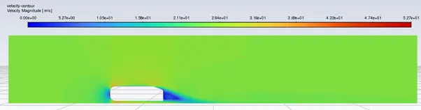
Velocity contour
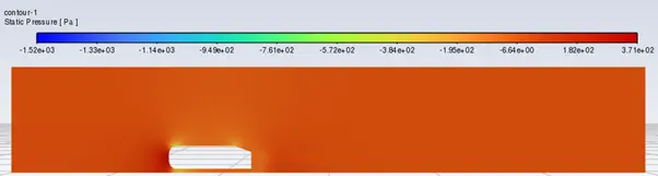
Pressure contour
Vector plot
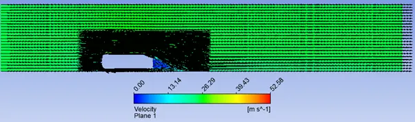
Wake region
Case – 4
For bigger Enclosure
Mesh element size = 85mm
Maximum size = 100mm
Inflation (car wall) no. of layers = 6
Growth rate = 1.2
Inflation option = first layer thickness
First layer thickness = 1.4mm
For smaller Enclosure
Body sizing
Element size = 65mm
Face sizing bottom leg
Element size = 5mm
No. of nodes = 56914
No. of elements = 135806
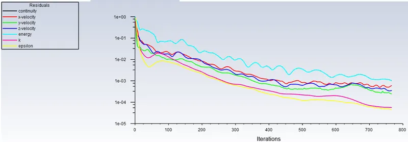
Residuals
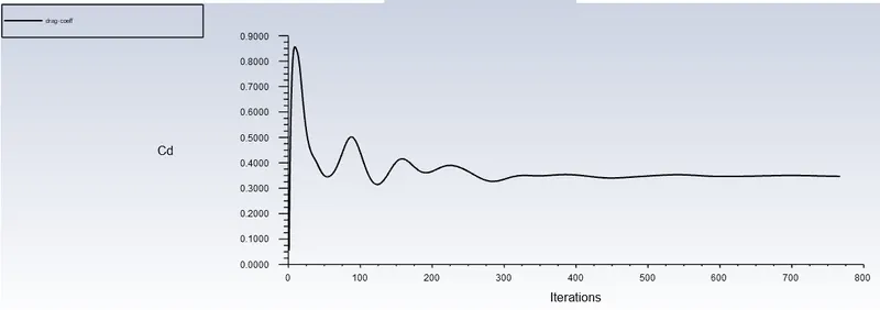
Coefficient of drag
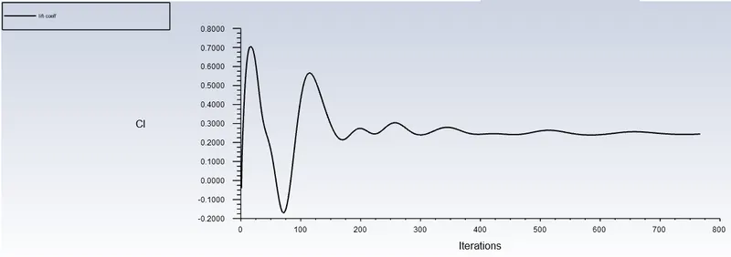
Coefficient of lift
Velocity contour
Pressure contour
Vector plot
wake region
Comparison table
|
Y+ |
`Y_p` (mm) |
Outer box mesh size (mm) |
Inner box mesh size (mm) |
Drag coefficient |
Lift coefficient |
|
100 |
1.4 |
100 |
100 |
0.39 |
0.29 |
|
100 |
1.4 |
85 |
65 |
0.35 |
0.24 |
|
100 |
1.4 |
80 |
60 |
0.33 |
0.25 |
|
100 |
1.4 |
60 |
50 |
0.31 |
0.27 |
Conclusion
- We can observe that the value of the coefficient of drag is reducing and the coefficient of lift is increasing (except first case) as we are refining the grid size this is happening because we are refining near walls of the car body based on y + values.
- In the wake reason we can see that there is a formation of recirculation zone due to boundary layer separation at the back of the body.
- All the case studies performed by considering the velocity of 25 m/sec. it is expected to see that an increase in velocity will cause boundary layer separation near the beginning of the slant surface and more vertex formation at the back of a body
- Study of static pressure contour help us in understanding the sudden deceleration of flow and red color indicates that static pressure raises the front of the body.
Reference
https://www.researchgate.net/publication/330383775_Experiments_and_numerical_simulations_on_the_aerodynamics_of_the_Ahmed_body