Week - 3 Drop test Challenge

Cell Phone Drop Test Analysis Using LS Dyna

by Swaroop Kumar Nagnoor

Problem Statement:

An Input file containing the FE Model of Cell Phone and the ground (Plate) is supplied. Drop Test Analysis has to be performed for the provided Cell Phone model by performing entire deck setup and analysis along with postprocessing of the results.

Aim:

To perform Drop test for a Cell phone model using LS Dyna

Objectives:

• Complete deck setup using *INITIAL_VELOCITY card and other appropriate keywords and controls in LS-PrePost
• Analysis using LS-DYNA Analysis
• Post-processing of results using LS-PrePost

Explanation:

Importing the FE Model:

• Launch LS-Dyna Program Manager
• Open LS-PrePost from the toolbar
• In LS-PrePost, open the FE Model from File-> Open-> LS-DYNA Keyword File

FE Model Clean-up:

• Once the model is imported, we can see that there is a total of 3 parts in the model; 1 shell plate with Part-ID-1and 2 solid plates with Part-ID-3 and Part-ID-4

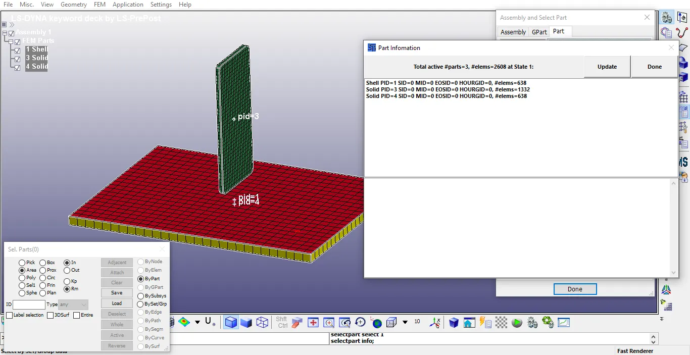
Figure 1: FE Model Input from keyword file

• Cell phone is represented by Part-ID-3
• The plate mimicking the ground can be represented either by solid elements (Part-ID-4) or by shell elements (Part-ID-1)
• Since in the model both the type of elements is present, we make use of the solid elements and delete the shell elements (Part-ID-1) to reduce the model complexity and maintain consistency

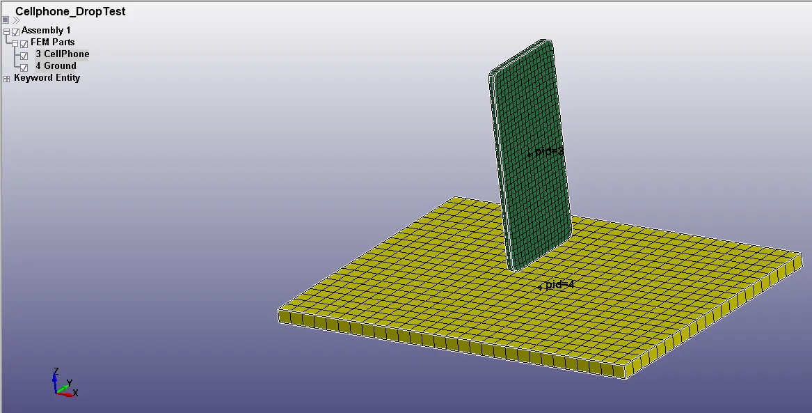
Figure 2: FE Model after Clean-up

Material Creation:

• For Ground plate, 020-MAT_RIGID material is considered

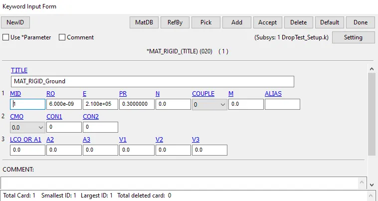
Figure 3: Material Card for Ground Plate

• Since no material details for the cell phone are available, 024-PIECEWISE_LINEAR_PLASTICITY material is considered with assumed values of density, young’s modulus and Poisson’s ratio

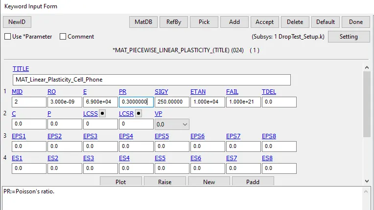
Figure 4: Material Card for Cell Phone

Defining Section:

• Since all the elements in the current analysis are Solid, a *SECTION_SOLID card is defined with the corresponding properties

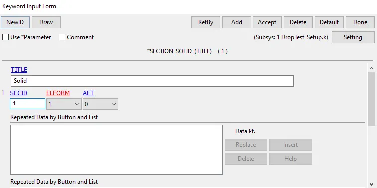
Figure 5: Solid Section Definition

Updating the Parts:

• Once the material type and the section type are defined, we have to update the same properties to the parts containing those elements

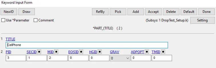
Figure 6: Properties updation for Cell Phone

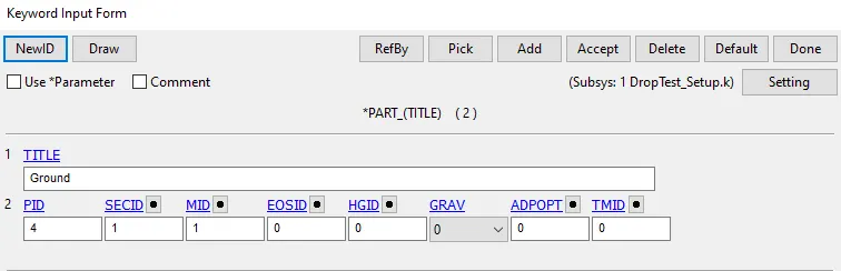
Figure 7: Properties updation for Ground

Boundary Conditions:

• A NODE_SET is created from the bottom nodes of the ground plate and constraints are applied to this node set in all 6DOF (Since it is a Solid type element, the nodes do not have any free rotational DOF and hence constraining the bottom nodes in 3 Translational DOF will also result in same effect)

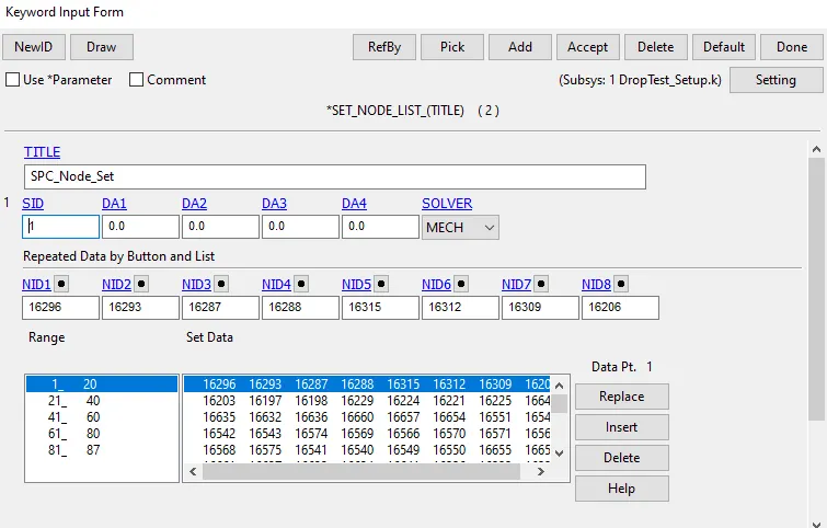
Figure 8: Node Set for Ground (SPC)

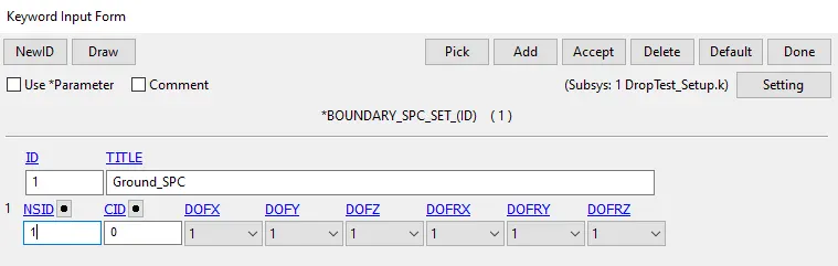
Figure 9: SPC Boundary Condition for Ground

Loading:

• In a Drop test, the Cell Phone is expected to freely fall from a certain height as prescribed by the manufacturer
• Since the data for the same is not available, we assume that the cellphone is already in motion and is travelling with some initial velocity. We define this initial velocity parameter as our only loading along with the default gravity loading for our analysis.
• All the nodes of the Cell Phone are expected to be travelling with the same velocity and hence a NODE_SET is created for these nodes and the *INITIAL_VELOCITY loading is then assigned.

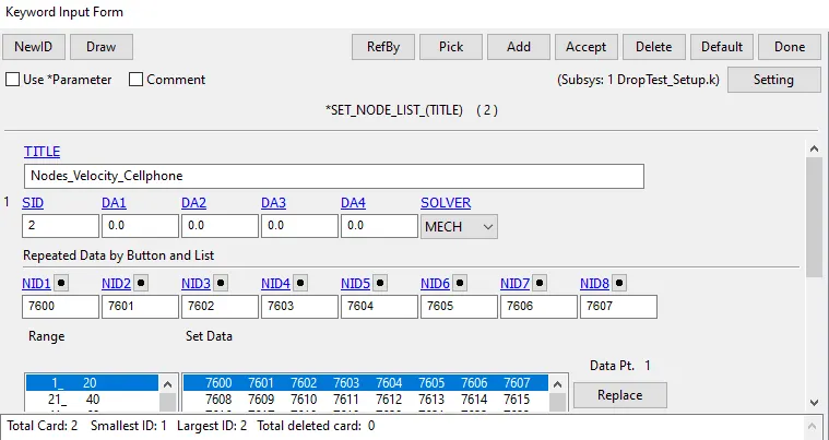
Figure 10: Node Set for Cell Phone

• The value for the initial velocity is based on the calculation assuming that the cell phone will take approximately 3 milli-seconds to hit the ground

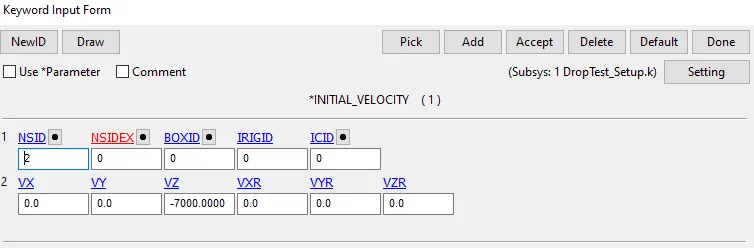
Figure 11: Defining INITIAL VELOCITY for Cell Phone

Contact Definition:

• A simple Automatic Surface to Surface contact is assumed in the current case where the deformable body (Cell Phone) is treated as a Slave and the undeformable body (Ground Plate) is treated as Master

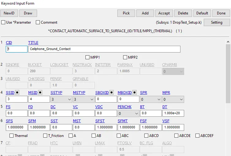
Figure 12: Contact Definition (Automatic Surface to Surface)

Control Cards:

• Control_Termination: Since the cell phone is expected to touch the ground in 3 milli-seconds, a total run time of 6 milli-seconds is considered for the current analysis
• Control_Hourglass: Default values used
• Control_Energy: Default values used

Output Database (dt = 0.0001):

• ASCII_Option
  • GLSTAT
  • MATSUM
  • RCFORC
  • SLEOUT
• BINARY_D3PLOT

Analysis:

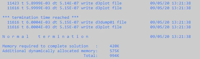
Figure 13: Analysis Output – Normal termination

Figure 14: Analysis Output – Run Time

Results:

• Load the results file (Binary file) into LS-PrePost
• A detailed review of the results is shown in the following Contours and Plots

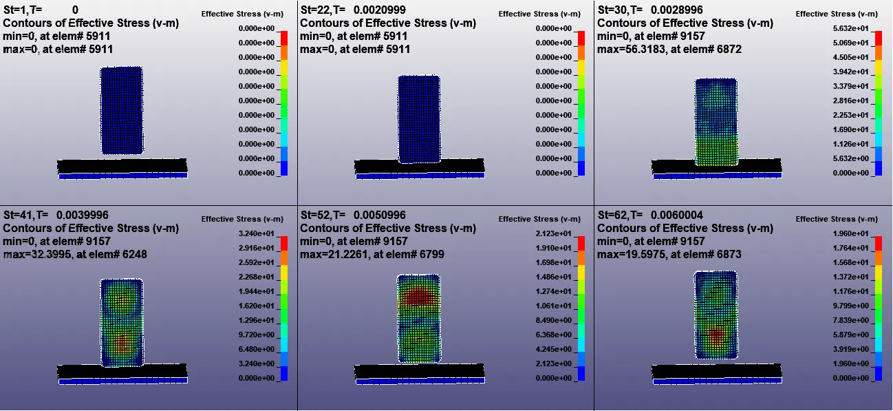
Figure 15: Effective Stress (vonMises) Contours at different timesteps

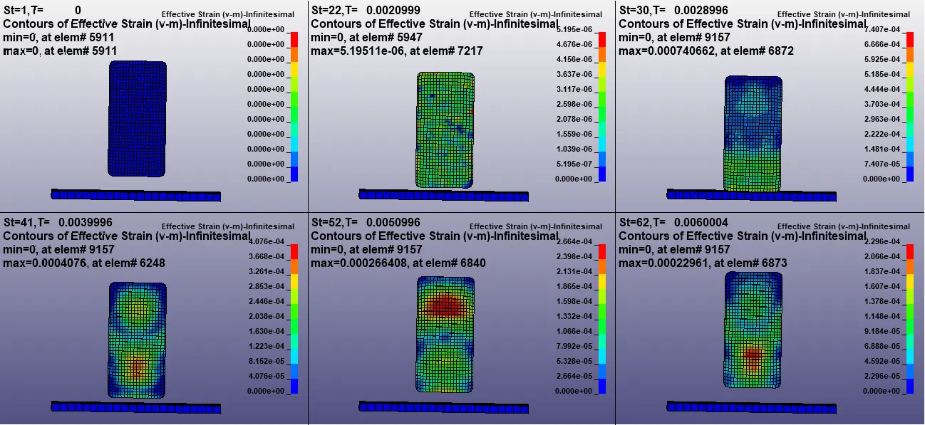
Figure 16: Effective Infinitesimal Strain (vonMises) Contours at different timesteps

• From the contours of Effective vonMises Stress and Effective Infinitesimal vonMises Strain, it is evident that the value of both Stress and Strain just after the impact (t = 0.00029 sec) is higher and tends to decrease thereafter. Also, a clear propagation of the Stress and Strain can be seen in the later time steps after the impact.

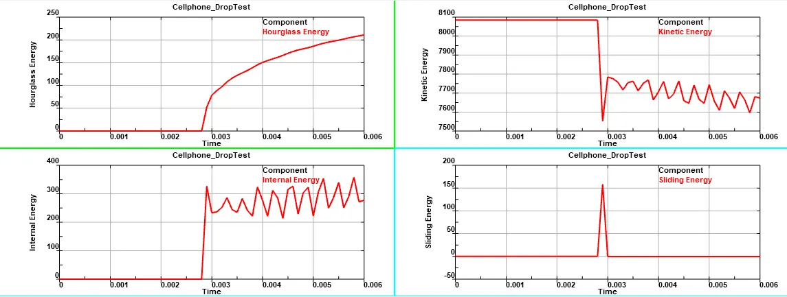
Figure 17: ASCII Output Plot- *GLSTAT

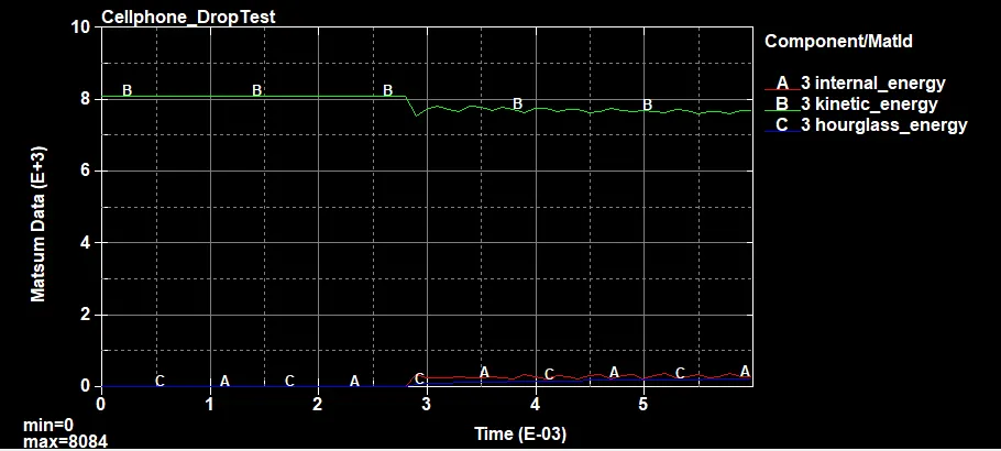
Figure 18: ASCII Output Plot- *MATSUM

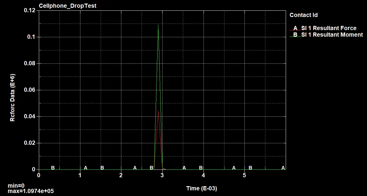
Figure 19: ASCII Output Plot- *RCFORC

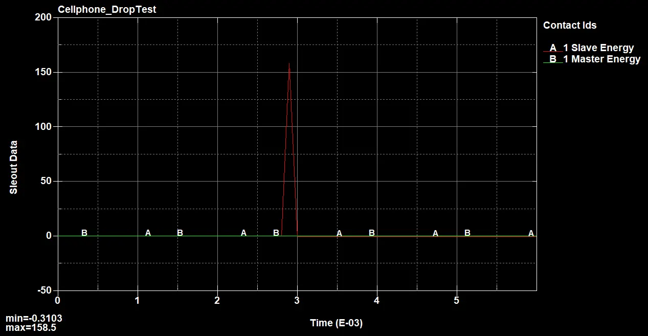
Figure 20: ASCII Output Plot- *SLEOUT

• From the above graphs, it can be seen that Hourglass Energy, and Internal Energy of the Component increases after the impact whereas the Kinetic energy decreases rapidly.
• The Resultant Forces and Moments on the component along with its Sliding Energy are non-zero during the contact and then drops back to zero.

Conclusion:

A Preliminary Drop-Test Analysis is performed on the Cell Phone model and its response over time was visualised. The objective of the analysis is hence accomplished and the same is documented.