Week - 2 - Explicit and Implicit Analysis

Nonlinear Static – Explicit and Implicit Analysis Example

by Swaroop Kumar Nagnoor

Problem Statement:

Consider the case of a simple bar in tension as shown in Figure 1. Suppose that the force in the bar is a nonlinear function of the displacement f(u) = u³ + 9u² + 4u. Solve the equation using both Explicit and Implicit Methods (Tolerance = 10^-2)

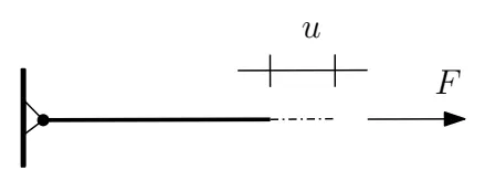
Figure 1: Bar in Tension

Aim:

To investigate the concept of Explicit and Implicit Methods applied to a case of simple bar in tension

Objectives:

• Displacement and Internal Force in the bar as a result of external Incremental load on the bar is calculated using both Explicit and Implicit Methods
• Residual (R) of the forces for each incremental load (Internal and External) is then calculated and checked if the value is within the specified tolerance limits

Procedure:

Force in the bar as a function of displacement is given by,

(1)

Stiffness of the bar from (1) is:

(2)

Explicit Analysis:

Five equal load increments (or steps) of ∆F = 1 unit each are used to load the tension bar.

Variables:

Displacement = u

internal force in the bar = f

external force applied to the bar = F

stiffness = k

Incremental displacements = ∆u

Incremental externally applied forces = ∆F (∆F = k*∆u)

Residual = R

Step 1
u₀ = 0.0

⇒ k(u₀) = = 4

∆F = 1

∆u₁ = = ¼ = 0.25

u₁ = u₀ + ∆u₁ = 0.25

f_int = f(u₁) = = 1.5781

F_ext = ∆F = 1

R = f_int - F_ext = 0.5781

||R|| > 10^-2 (Specified Tolerance)

Step 2
u₁ = 0.25

⇒ k(u₁) = = 8.6875

∆F = 1

∆u₂ = = 1/8.6875 = 0.1151

u₂ = u₁ + ∆u₂ = 0.3651

f_int = f(u₂) = = 2.7088

F_ext = ∆F + ∆F = 2

R = f_int - F_ext = 0.7088

||R|| > 10^-2 (Specified Tolerance)

Step 3

u₂ = 0.3651

⇒ k(u₂) = = 10.9719

∆F = 1

∆u₃ = = 1/10.9719 = 0.0911

u₃ = u₂ + ∆u₃ = 0.4563

f_int = f(u₃) = = 3.7935

F_ext = ∆F + ∆F + ∆F = 3

R = f_int - F_ext = 0.7935

||R|| > 10^-2 (Specified Tolerance)

Step 4

u₃ = 0.4563

⇒ k(u₃) = = 12.8370

∆F = 1

∆u₄ = = 1/12.8370 = 0.0779

u₄ = u₃ + ∆u₄ = 0.5342

f_int = f(u₄) = = 4.8568

F_ext = ∆F + ∆F + ∆F + ∆F = 4

R = f_int - F_ext = 0.8568

||R|| > 10^-2 (Specified Tolerance)

Step 5

u₄ = 0.5342

⇒ k(u₄) = = 14.4706

∆F = 1

∆u₅ = = 1/14.4706 = 0.0691

u₅ = u₄ + ∆u₅ = 0.6033

f_int = f(u₅) = = 5.9078

F_ext = ∆F + ∆F + ∆F + ∆F + ∆F = 5

R = f_int - F_ext = 0.9078

||R|| > 10^-2 (Specified Tolerance)

Hence, for external load increment of ∆F = 1 unit, it is evident that the external forces and internal forces are not in equilibrium because F_{ext ≠} f_int. Hence the curve for the explicit method is deviating away from the actual curve as shown in Figure 2.

To understand the reason for this drift, a smaller load increment of ∆F = 0.1 unit is considered. The curve for the explicit method with smaller load increments closely follows the actual curve. But still the tolerance condition is still not satisfied as the norm of Residual ||R|| > 10^-2.

Hence, as per the definition of Explicit Methods, a smaller step size results in a stable computation as the curve closely follows the actual data, whereas a larger step size leads to a solution divergence. However, both load steps fail to achieve the accuracy required by the solution.

Detailed summary and calculations of the results for Explicit analysis are shown in the attached spreadsheet.

Implicit Analysis:

The calculations for the implicit analysis are the same as the explicit analysis, except that at the end of each step Newton-Raphson iterations are used to enforce equilibrium before moving to the next step.

For a given step size or load increment, internal forces and external forces will be in equilibrium only when the stiffness is linear. To achieve this, corrections are made to the calculated displacement value in each step. This is achieved by Newton-Raphson iterations to minimize the residual (R(u) = f_int - F_ext).

From Taylors series for current displacement (neglecting higher order terms), the residual with correction is given by

(3)

⇒

⇒ (4)

Variables:

Displacement = u

internal force in the bar = f

external force applied to the bar = F

stiffness = k

Incremental displacements = ∆u

Incremental externally applied forces = ∆F (∆F = k*∆u)

Residual = R

Correction = δ

Step 1
u₀ = 0.0

⇒ k(u₀) = = 4

∆F = 1

∆u₁ = = ¼ = 0.25

u₁ = u₀ + ∆u₁ = 0.25

f_int = f(u₁) = = 1.5781

F_ext = ∆F = 1

R⁽⁰⁾ = f_int - F_ext = 0.5781

||R⁽⁰⁾|| > 10^-2, hence Newton-Raphson iterations are necessary

Step 1.1

For calculating the correction, = 0.25

Stiffness = = = 8.6875

Correction = = - [8.6875] * 0.5781 = -0.0665

Updated = 0.1835

f_int = f() = = 1.0429

F_ext = ∆F = 1

R⁽¹⁾ = f_int - F_ext = 0.0429

||R⁽¹⁾|| > 10^-2, hence another Newton-Raphson iteration is necessary

Step 1.2

For calculating the correction, = 0.1835

Stiffness = = = 7.4031

Correction = = - [7.4031] * 0.0429 = -0.0058

Updated = 0.1777

f_int = f() = = 1.0003

F_ext = ∆F = 1

R⁽²⁾ = f_int - F_ext = 0.0003

||R⁽²⁾|| < 10^-2, hence no further iterations are necessary

Hence u₁ = 0.1777;

Step 2
u₁ = 0.1777

⇒ k(u₁) = = 7.2926

∆F = 1

∆u₂ = = 1/7.2926 = 0.1371

u₂ = u₁ + ∆u₂ = 0.3148

f_int = f(u₂) = = 2.1822

F_ext = ∆F + ∆F = 2

R⁽⁰⁾ = f_int - F_ext = 0.1822

||R⁽⁰⁾|| > 10^-2, hence Newton-Raphson iterations are necessary

Step 2.1

For calculating the correction, = 0.3148

Stiffness = = = 9.9634

Correction = = - [9.9634] * 0.1822 = -0.0183

Updated = 0.2965

f_int = f() = = 2.0033

F_ext = ∆F + ∆F = 2

R⁽¹⁾ = f_int - F_ext = 0.0033

||R⁽¹⁾|| < 10^-2, hence no further iterations are necessary

Hence u₂ = 0.2965;

Step 3
u₂ = 0.2965

⇒ k(u₂) = = 9.6007

∆F = 1

∆u₃ = = 1/9.6007 = 0.1042

u₃ = u₂ + ∆u₃ = 0.4007

f_int = f(u₃) = = 3.1117

F_ext = ∆F + ∆F + ∆F = 3

R⁽⁰⁾ = f_int - F_ext = 0.1117

||R⁽⁰⁾|| > 10^-2, hence Newton-Raphson iterations are necessary

Step 3.1

For calculating the correction, = 0.4007

Stiffness = = = 11.6934

Correction = = - [11.6934] * 0.1117 = -0.0096

Updated = 0.3911

f_int = f() = = 3.0009

F_ext = ∆F + ∆F + ∆F = 3

R⁽¹⁾ = f_int - F_ext = 0.0009

||R⁽²⁾|| < 10^-2, hence no further iterations are necessary

Hence u₃ = 0.3911;

Step 4
u₃ = 0.3911

⇒ k(u₃) = = 11.4987

∆F = 1

∆u₄ = = 1/11.4987 = 0.0870

u₄ = u₃ + ∆u₄ = 0.4781

f_int = f(u₄) = = 4.0785

F_ext = ∆F + ∆F + ∆F + ∆F = 4

R⁽⁰⁾ = f_int - F_ext = 0.0785

||R⁽⁰⁾|| > 10^-2, hence Newton-Raphson iterations are necessary

Step 4.1

For calculating the correction, = 0.4781

Stiffness = = = 13.2908

Correction = = - [13.2908] * 0.0785 = -0.0059

Updated = 0.4722

f_int = f() = = 4.0004

F_ext = ∆F + ∆F + ∆F + ∆F = 4

R⁽¹⁾ = f_int - F_ext = 0.0004

||R⁽²⁾|| < 10^-2, hence no further iterations are necessary

Hence u₄ = 0.4722;

Step 5
u₄ = 0.4722

⇒ k(u₄) = = 13.1685

∆F = 1

∆u₅ = = 1/13.1685 = 0.0759

u₅ = u₄ + ∆u₅ = 0.5481

f_int = f(u₅) = = 5.0614

F_ext = ∆F + ∆F + ∆F + ∆F + ∆F = 5

R⁽⁰⁾ = f_int - F_ext = 0.0614

||R⁽⁰⁾|| > 10^-2, hence Newton-Raphson iterations are necessary

Step 5.1

For calculating the correction, = 0.5481

Stiffness = = = 14.7679

Correction = = - [14.7679] * 0.0614 = -0.0042

Updated = 0.5440

f_int = f() = = 5.0002

F_ext = ∆F + ∆F + ∆F + ∆F + ∆F = 5

R⁽¹⁾ = f_int - F_ext = 0.0002

||R⁽²⁾|| < 10^-2, hence no further iterations are necessary

Hence u₅ = 0.5440;

It is evident from the above computations that the external forces and internal forces are coming into equilibrium. Hence the system is stable.

Hence, as per the definition of Implicit Methods, the solution is stable and accurate even for large step size, but the number of computations required to complete each iteration are higher than that of the explicit method.

In Figure 2, the curve for the implicit method exactly overlaps with the actual curve.

Detailed summary and calculations of the results for Implicit analysis is shown in the attached spreadsheet.

Discussion on result plots:

• A plot of the results is shown in Figure 2.
• For an external load increment of ∆F = 1 unit, the curve for the explicit method is deviating away from the actual curve as the external forces and internal forces are not in equilibrium because F_{ext ≠} f_int. and the residual value is far away from the specified tolerance limit on the higher side.
• For a smaller load increment of ∆F = 0.1 unit, the explicit analysis more closely follows the exact solution as shown in Figure 3.
• However, even with more increments the explicit analysis still drifts from the exact solution as the residual is not within the specified tolerance.
• The drift from the exact solution illustrates the lack of equilibrium between the internal and external forces.
• To correct for this problem an implicit analysis is required.
• The results for the implicit analysis are shown in Figure 2.
• The Newton-Raphson iterations correct the incremental steps such that they coincide with the exact solution and the residual is within the specified tolerance.

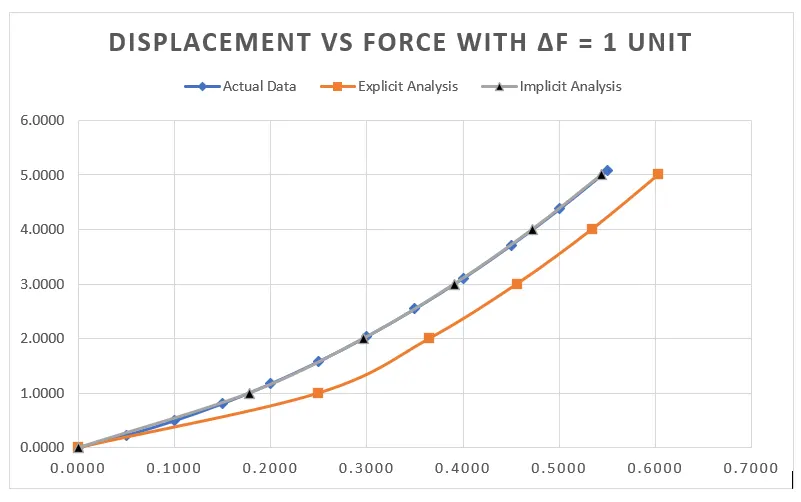
Figure 2: Comparison of Explicit, Implicit and Exact results of load versus displacement

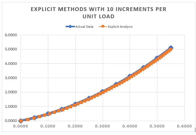
Figure 3: Explicit results using smaller load step ∆F = 0.1 Unit

(10 Increments per unit load)

Conclusion:

For the nonlinear analysis on a simple bar, computations are performed using both implicit and explicit schemes and the results for the same are plotted and compared. The Explicit scheme does not favour the calculations as the results are drifting away from the actual case. Whereas the Implicit Scheme satisfies all the conditions and the computations match very well with the actual curve. Hence, for this particular case where load increment is considered as the criteria, Implicit Scheme is predominant and advantageous over the Explicit Scheme in terms of stability and accuracy.