Week-3 Challenge: ADVISOR Tool

INTRODUCTION:

What is an advisor?

Advanced Vehicle Simulator was first developed in November 1994 at the National Renewable Energy Laboratory. It was designed as an analysis tool to assist the US Department of Energy(DOE) in developing technologies for hybrid electric vehicles through the hybrid electric propulsion system contracts with Ford, General Motors, and DaimlerChrysler. Its primary role is to highlight the system-level interactions of hybrid and electric vehicle components and their impacts on the vehicle's performance and fuel economy.

ADVISOR was created in MATLAB/SIMULINK environment. MATLAB provides an easy-to-use matrix-based programming environment for calculations, while Simulink can be used to represent complex systems graphically using block diagrams. ADVISOR uses three primarily graphical user interface(GUI) screens to guide the user through the simulation process. With the GUIs, the user can iteratively evaluate the impacts of vehicle parameters and drive cycle requirements on vehicle performance, fuel economy, and emissions. The GUIs facilitate interaction with the raw input and output data that is present in the MATLAB workspace. The component data is stored in the form of text files, and based on the user's selections, the appropriate data sets are loaded into the workspace. The two most common uses of the ADVISOR are for drive-cycle analysis and performance analysis.

ADVISOR Approach:

Advisor uses a hybrid backward/forward approach that is closely related to the strictly backward-facing approach. ADVISOR approach is unique in the way it handles the component performance limits in its backward-facing stream of calculations and in the addition of forward-facing stream of calculations.

Generic Backward-facing approach:

Vehicle simulators using a backward-facing approach answer the question ‘‘assuming the vehicle met the required trace, how must each component perform?’’ No model of driver behavior is required in such models. Instead, the force required to accelerate the vehicle through the time step is calculated directly from the required speed trace. The required force is then translated into a torque that must be provided by the component directly upstream, and the vehicle’s linear speed is likewise translated into a required rotational speed. Component by component, this calculation approach carries backward through the drivetrain, against the tractive power flow direction, until the fuel use or electrical energy use that would be necessary to meet the trace is computed. The backward-facing approach is convenient because automotive drivetrain components tend to be tested in a laboratory environment such that a table of efficiency or loss versus output torque and speed (or power) is developed. This means that a straightforward calculation can determine a component’s efficiency and allow the calculation to progress. The explicit nature of the efficiency/loss calculation also allows very simple integration routines (e.g. Euler) to be used with relatively large time steps on the order of 1 s. Thus, simulations using the backward-facing approach tend to execute quickly. Weaknesses of the backward-facing approach come from its assumption that the trace is met and from the use of efficiency or loss maps. Since the backward-facing approach assumes that the trace is met, this approach is not well suited to compute best-effort performance, such as occurs when the accelerations of the speed trace exceed the capabilities of
the drivetrain. Also, because efficiency maps are generally produced by steady-state testing, dynamic effects are not included in the maps or in the backward-facing model’s estimate of energy use. A related limitation of the backward-facing model is that it does not deal with the quantities directly measurable in a vehicle. For example, control signals such as throttle and brake position are absent from the model, further hindering dynamic system simulation and detailed control system development.

Generic Forward-facing approach:

Vehicle simulators that use a forward-facing approach include a driver model, which considers the required speed and the present speed to develop appropriate throttle and brake commands (often through a PI controller). The throttle command is then translated into a torque provided by the engine (and/or motor) and an energy use rate. The torque provided by the engine is input to the transmission model, which transforms the torque according to the transmission’s efficiency and gear ratio. In turn, the computed torque is passed forward through the drivetrain, in the direction of the physical power flow in the vehicle, until it results in a tractive force at the tire/road interface. The resultant acceleration is computed from an ¼F/meff,
where meff includes the effect of rotational inertia in the drivetrain. The forward-facing approach is particularly desirable for hardware development and detailed control simulation. Since forward-facing models deal in quantities measurable in the latest drivetrain, such as control signals and true torques (not torque ‘requirements’), vehicle controllers can be developed and tested effectively in simulations. Also, dynamic models can be included naturally in a forward-facing vehicle model. Finally, the forward-facing approach is well-suited to the calculation of maximum effort accelerations, as they are essentially wide-open throttle events. The major weakness of the forward-facing approach is its simulation speed. Drivetrain power calculations rely on the vehicle states, including drivetrain component speeds that are computed by integration. Therefore, higher-order integration schemes using relatively small-time steps are necessary to provide stable and accurate simulation results. As a result, forward-facing simulation can be overly time-consuming for use in preliminary design studies.

AIM:

Use the ADVISOR tool and simulate the following.

OBJECTIVE:

1. For the EV_defaults_in file, if the cargo mass is 500 kg with all other default conditions, can the vehicle travel for 45 km with an FTP drive cycle? Conclude your observations.

Here we have to check whether the EV model with a cargo mass of 500 kg can travel 45 km with an FTP drive cycle pattern of acceleration and deceleration.

Firstly, we have to open the ADVISOR window by just typing the ADVISOR in the MATLAB command window. An input GUI window of ADVISOR pops up. This window shows a default parallel hybrid model, using a drop-down menu, EV_default_in model file, to perform the analysis. Furthermore, the Cargo mass should be changed to 500 kg, then continue to the next GUI interface where one can select the type of drive cycle (here FTP drive cycle). Then the model with these parameter changes should be run for simulation. The simulation should be checked iteratively until the SOC of the battery is zero. Then the total range of the vehicle has resulted from the results GUI window.

In my analysis, I have been increasing the drive cycles until the SOC of the Battery is zero. Each drive cycle takes, 2477s to complete one cycle. With the cargo, the mass increased, and the range of the vehicle decreased compared to the default mass of the vehicle model.

1. EV_default_in model with cargo mass 500 kg. Here one can change the input parameters manually according to required condition of the model.

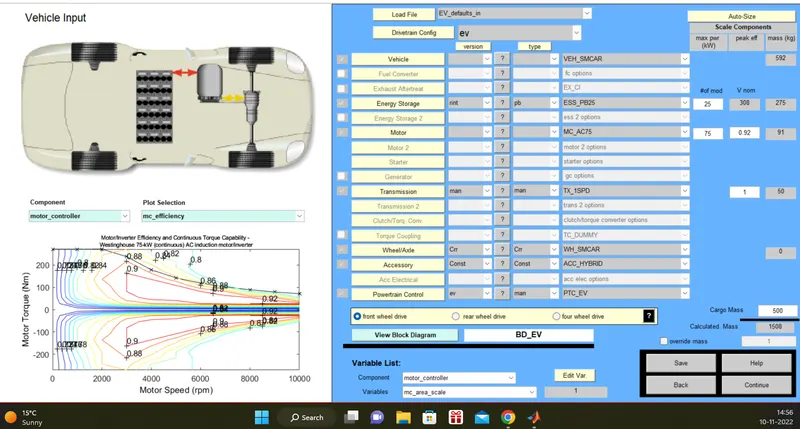
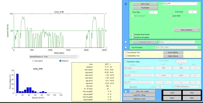
2. Once the continue button is pressed, the second GUI opens up, it is called Simulation parameters. One can select the type of drive cycle the model performance should be analyzed, grade percentage can also be changed, and acceleration time can be assessed by giving conditions. Here FTP drive cycle is chosen for the analysis.

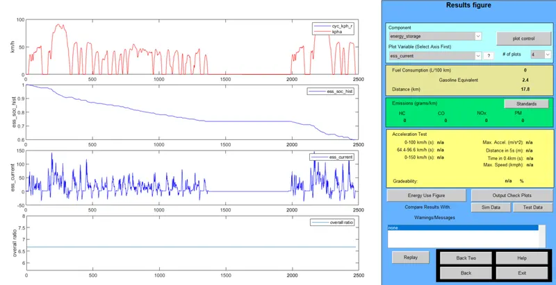
3. Results plots are the final GUI that popped up, here we can observe the model behavior to the condition parameters. With one FTP drive cycle, the EV model has traveled a 17.8 KM distance with still approx 0.6 % of the total charge in the battery left, and thus we continue the same iterative simulation by increasing the driving cycles until SOC is zero.

Observation:

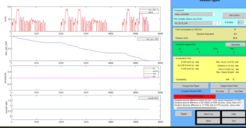
The above EV vehicle model with two FTP drive cycles traveling for 4594s can cover the range of p to 35.6 Km and still approx 0.3% of the charge left in the battery. Again, another FTP cycle is added to increase the time of travel, final results are as the vehicle couldn't complete the 3rd cycle due to zero energy source. SOC of the battery reached zero, and the total range of the vehicle is 41.4 Km.

Conclusion:

Therefore, EV_default cannot travel a distance of 45 KM in an FTP drive cycle with a payload of 500 kg.

2. In the above case, try changing the battery capacity and repeat the simulation.

In the above analysis 1, it is observed that the mass parameter of the vehicle is changed to 500 kg. With this payload and the battery capacity, the vehicle range was limited to 41.4 km in the FTP drive cycle pattern. Now, in the current analysis, the battery capacity is increased accordingly to meet the required range of 45 km. Now the iterative process is again carried out to check what capacity is optimum to get desired range of the vehicle.

In the default model, we have a battery with 25 modules and a nominal voltage of 308 volts. With this parameter definition, the vehicle was able to travel only 41.4 km. In the first iterative step, we will increase the number of modules to 27 with 333 volts nominal voltage and check whether we get the desired range.

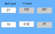
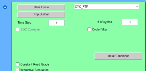
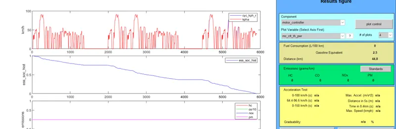
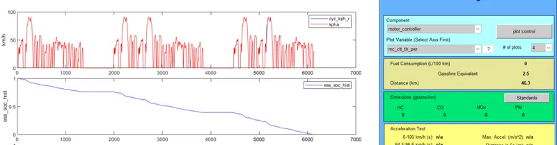
In the picture, we can observe that the vehicle SOC is zero after 3 driving cycles with 27 modules and 333 volts voltage. Still, the desired range cannot be reached. Thus, we can increase the battery capacity a bit to get desired range.

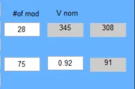
Now I choose to increase the battery modules to 28 with 345 volts of nominal voltage.

Conclusion:

Thus from the iterative analysis, we can see that the EV model design carrying a 500 kg Payload requires 28 modules of the battery with 345 Volts of nominal voltage to reach the range of 45 Km. With this type of battery configuration, we cannot exceed the range above 46.3 km.

3. Perform gradeability test with PRIUS_Jpn_defaults_in file

Gradeability is defined as the ability of a vehicle to ascend the upslope at a constant speed without stalling.

In this analysis, we have to quantify the Gradeability percentage that the Prius can overcome with an increase in speeds during ascending the slope for a certain time period.

Below is the input window of the Prius model. The model Prius should be selected from the drop-down menu and further all other parameters are kept unchanged.

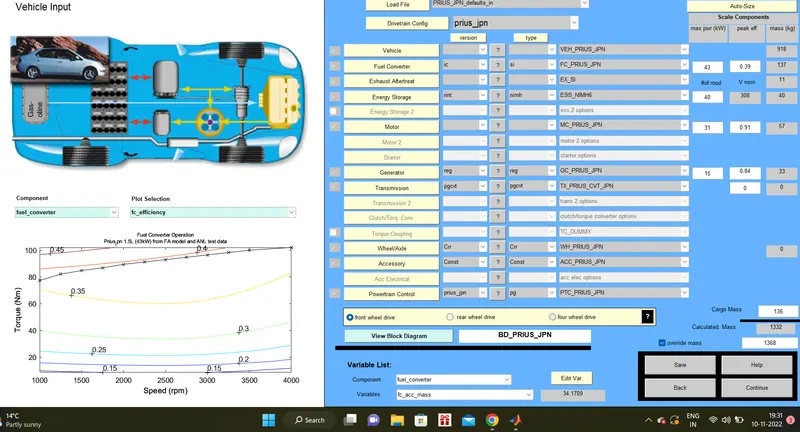
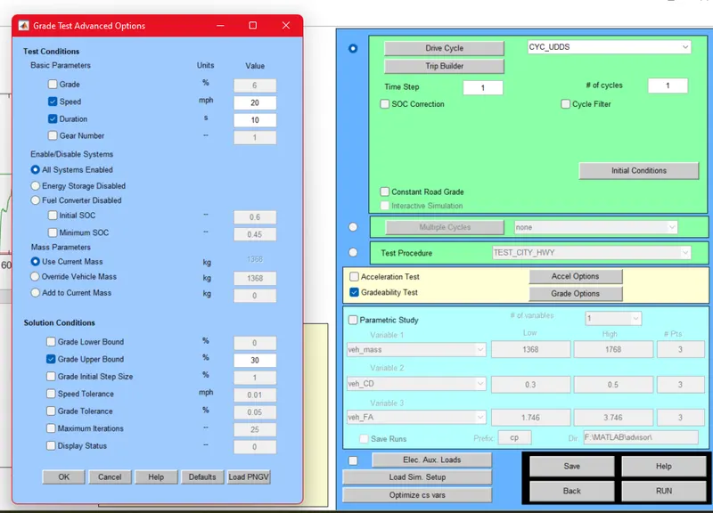
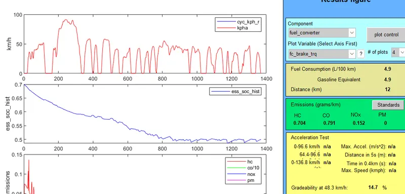
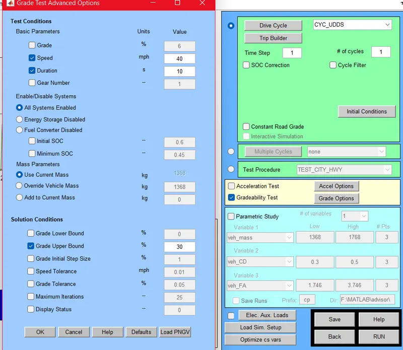
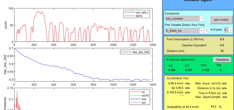
1. Let us consider the time period as 10s and keep increasing the speed in the steps of 10 mph for 4 cases. We are using UDDS drive for the gradeability analysis.

a) 20 mph - 32.2km/h the Gradeability is 19.8%.

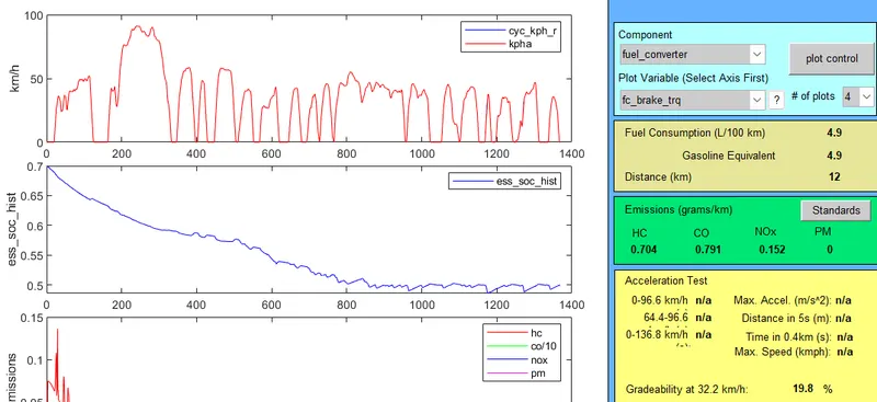
b) 20 mph - 48 km/h Gradeability = 14.7%

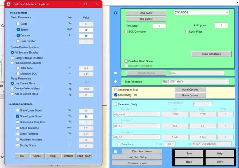
c) 40 mph - 64.4 km/h Gradeability 11.7%

d) 50 mph - 80.5 km/h Gradeability = 9.7%

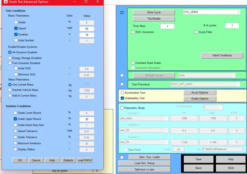
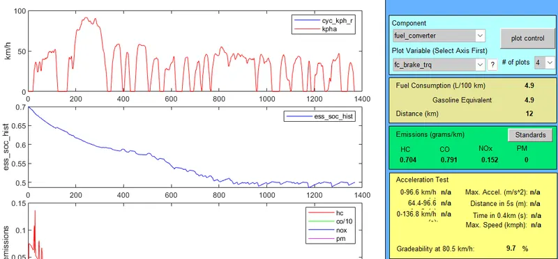
A similar iterative analysis is conducted for the same speeds but for a 20s time period. The results are updated below in the table.

Speed (mph)	Speed(km/h)	Time period (seconds)	Gradeability (%)
20	32.2	10	19.8
30	48.3	10	14.7
40	64.4	10	11.7
50	80.5	10	9.7

Speed (mph)	Speed(km/h)	Time period (seconds)	Gradeability (%)
20	32.2	20	22.5
30	48.3	20	16.3
40	64.4	20	13.5
50	80.5	20	10.8

Conclusion:

From the results, it can be observed that a steeper uphill slope results in confining the speed to a smaller speed interval. Similarly, steeper downhill grades result in higher speed distributions. Hence, we can conclude that a steeper gradient of an upslope reduces the speed, while a downslope increases a vehicle's velocity.