Week-3 Challenge: ADVISOR Tool

ADVISOR TOOL :

It is a set of model, data, and script text files for use with MATLAB and Simulink environment. This tool stands for 'Advanced Vehicle Simulator' which is used to model different types of vehicles such as some IC engine based and electric vehicles, hybrid vehicles and fuel cell-based vehicles, so this tool is very useful in case of user-defined powertrain/vehicle dynamics and wants to see the following results before the implementation of the model.

1. EV_defaults_in file with cargo mass= 500 kg :

Here, we have to check whether the vehicle can travel for 45 km with FTP drive cycle, having a cargo mass of 500 kg. At first, load the ADVISOR tool from the MATLAB command window and select the metric system, instead of the US system and load the EV_defaults_in file, where the cargo mass is changed to 500 kg, so the total calculated mass becomes 1508 kg and the remaining parameter values remain unchanged, as in fig 1.0. Then, hit the continue button to load the next GUI(Graphical User Interface).

fig 1.0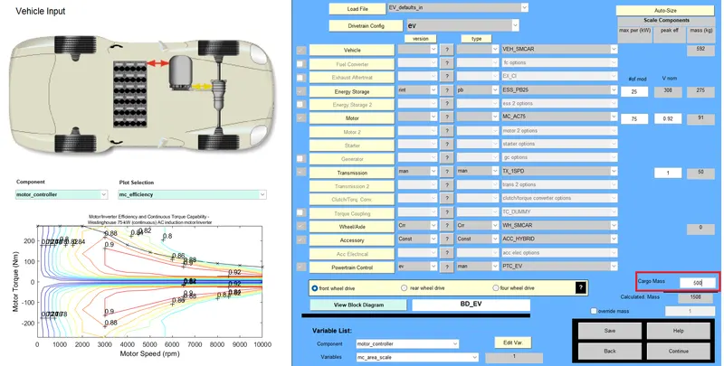

Here, we are using a FTP based drive cycle from the drive cycle option and the number of cycles is set at 1, as in fig 1.1. Then, the run is clicked to go to the next stage.

fig 1.1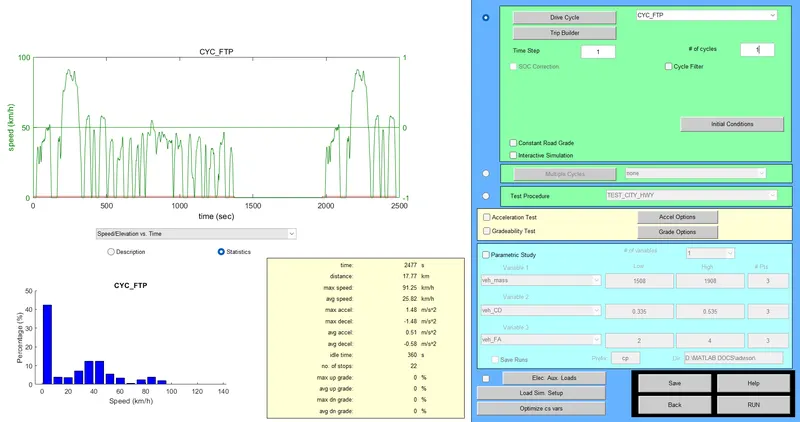

As, we run the previous GUI of the ev_default_in file with a single FTP cycle, it is seen that the distance(in km) covered is 17.8 km, which is very much less than the distance to be travelled(ie, 45 km), as in fig 1.2.

fig 1.2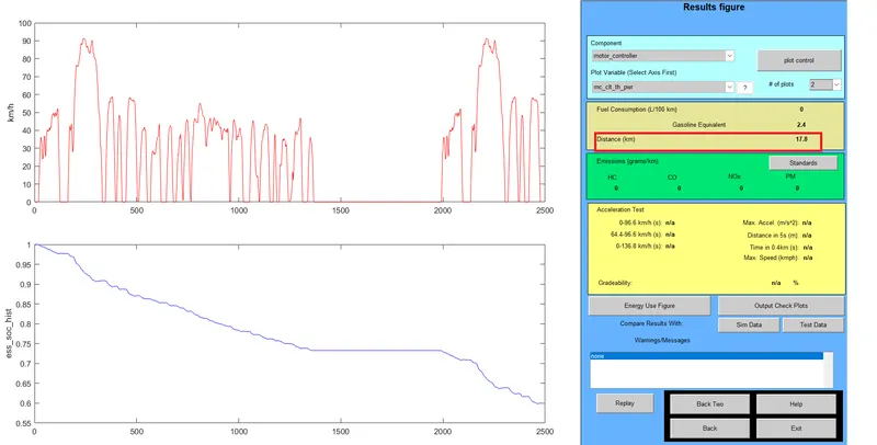

Here, in this case more than 1 drive cycle is required, so 3 drive cycles are taken into account and the it is again run. But, a warning is popped up indicating that the required distance exceeds the EV range, ie the distance that the vehicle can cover within the 3 cycles of FTP drive-cycles is 41.4 km, which is less than the required distance of 45 km; by a difference of 3.2 km at full battery capacity value of 25kW (ess_SOC = 100%), as in fig 1.3.

fig 1.3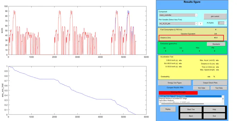

CONCLUSION :

Here, for 3 number of FTP drive-cycles; the total distance travelled is 41.4 km at the given conditions with 100% SOC value, less than the required distance. So, the vehicle model cannot travel the required distance of 45 km with the current battery capacity and in the given conditions.

2. Changing the battery capacity :

Here, the battery capacity is changed form 25 kW to 50 kW for the above ev_defaults_in file for the same cargo mass of 500 kg, which in turn increases the calculated mass from 1508 kg to 1783 kg, so that it can cover the distance of 45 km and the continue button is selected as in fig 2.0.

fig 2.0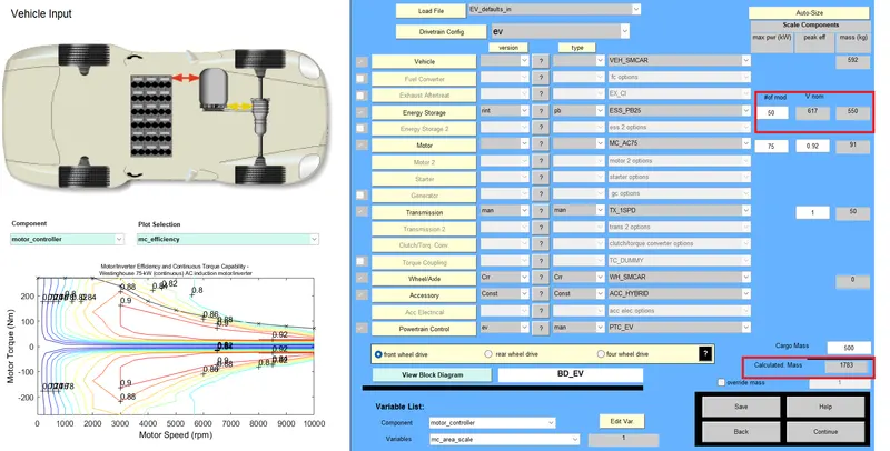

Also, in this case more than 1 drive cycle is required, so 3 drive cycles are taken into account to meet the required distance of 45 km and the it is again run. Here, it is seen that no warnings are given as the distance that the vehicle can cover within the 3 cycles of FTP drive-cycles is 53.3 km, which is much greater than the required distance of 45 km and it will not use the full battery capacity of 50 kW (ess_SOC = 90-95 %), as in fig 2.1.

fig 2.1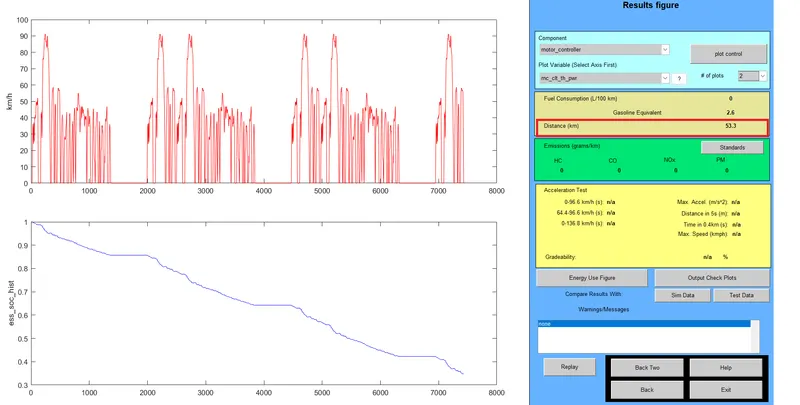

CONCLUSION :

Here, we see that when the battery capacity is increased from 25 kW to 50 kW, then the vehicle model covers the required distance of 45 km without using full battery capacity, ie SOC > 100%. Similarly, when we decrease the battery capacity, the vehicle model travels lesser distances.

3. To check the gradeability of PRIUS_Jpn_defaults_in file :

Here, we select the Prius_JPN_defaults_in file as the vehicle file from the load file option and the prius model file is loaded. All the default parameters are remained unchanged (fig 3.0) and the continue button is selected.

fig 3.0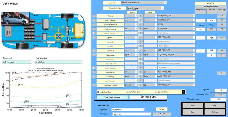

Here, inorder to check the gradeabitity of the prius_jpn_defaults file; here a UUDS cycle is selected as the drive cycle and the number of drive cycles is selected as 1 (any cycle/number of cycles can be selected as it is not specified in the question; I selected UDDS cycle and 1 cycle in number for simplicity purposes). As gradeabitity test is to be performed, so this option is selected and grade options are selected, where we need to change the option which will include both fuel and storage systems. Hence, we select the option: 'all systems enabled' and the speed option is changed on the range of your own observations; ie here, I am selecting the speed range as 10-50 mph(miles/hr) for a duration of 10 sec. Then, it is run for a total of 12 km.

(a) For a speed of 10 mph = 10*1.609 = 16.09 kmph :

Here, the speed in the grade options of a gradeability test is selected as 10 mph; so the gradeability at 16.1 km/hr is 30.3% (fig 3.1).

fig 3.1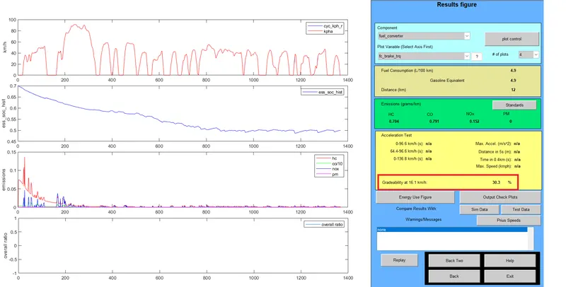

(b) For a speed of 20 mph = 20*1.609 = 32.18 kmph :

Here, the speed in the grade options of a gradeability test is selected as 20 mph; so the gradeability at 32.2 km/hr is 19.8% (fig 3.2).

fig 3.2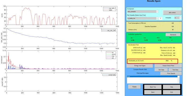

(c) For a speed of 30 mph = 30*1.609 = 48.27 kmph :

Here, the speed in the grade options of a gradeability test is selected as 30 mph; so the gradeability at 48.3 km/hr is 14.7% (fig 3.3).

fig 3.3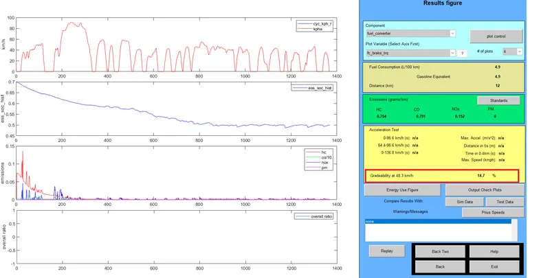

(d) For a speed of 40 mph = 40*1.609 = 64.36 kmph :

Here, the speed in the grade options of a gradeability test is selected as 40 mph; so the gradeability at 64.4 km/hr is 11.7% (fig 3.4).

fig 3.4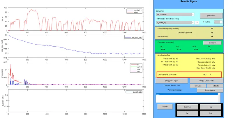

(d) For a speed of 50 mph = 50*1.609 = 80.45 kmph :

Here, the speed in the grade options of a gradeability test is selected as 50 mph; so the gradeability at 80.5 km/hr is 9.7% (fig 3.5).

fig 3.5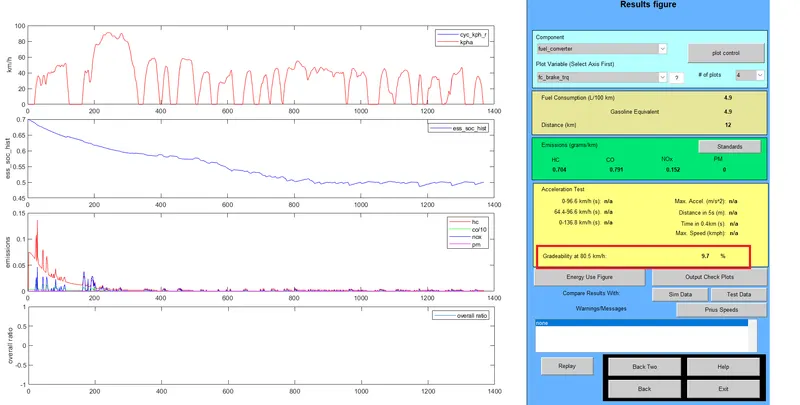

SL.NO	SPEED(in mph)	SPEED(in kmph)	GRADEABILITY(in %)
1.	10	16.1	30.3
2.	20	32.2	19.8
3.	30	48.3	14.7
4.	40	64.4	11.7
5.	50	80.5	9.7

CONCLUSION :

From the above table, it is seen that gradeability decreases with the increase in speed. So, in our observation, the gradeability will be the highest at 10 mph and the lowest at 50 mph.