Using ADVISOR Tool for basic simulations.

Using the Advisor tool to simulate various vehicle configurations.

Aim: The aim of the challenge is to use the Advisor tool and Simulate the default EV vehicle and a PRIUS_Jpn_defaults_in file for various test conditions.

Objective:

1. To increase the Load to 500kg for the Default Electric vehicle and see if the vehicle can travel for 45km with the FTP drive cycle.
2. Also, see the change in distance traveled when the batter is capacity is increased.
3. To perform the Gradability test with PRIUS_Jpn_defaults_in file.

Procedure:

ADVISOR, NREL’s ADvanced VehIcle SimulatOR, is a set of models, data, and script text files for use with Matlab and Simulink. It is designed for rapid analysis of the performance and fuel economy of conventional, electric, and hybrid vehicles.

ADVISOR also provides a backbone for the detailed simulation and analysis of user-defined drivetrain components, a starting point of verified vehicle data and algorithms from which to take full advantage of the modeling flexibility of Simulink and analytic power of MATLAB.

You may benefit from using ADVISOR if you want to:

1. estimate the fuel economy of vehicles that have not yet been built
2. learn about how conventional, hybrid or electric vehicles use (and lose) energy throughout their drivetrains
3. compare relative tailpipe emissions produced on a number of cycles
4. evaluate an energy management strategy for your hybrid vehicle’s fuel converter

In general, the user takes two steps:

1. Define a vehicle using measured or estimated components and overall vehicle data.
2. Prescribe a speed versus time trace, along with road grade, that the vehicle must follow.

ADVISOR then puts the vehicle through its paces, making sure it meets the cycle to the best of its ability and measuring (or offering the opportunity to measure) just about every torque, speed, voltage, current, and power passed from one component to another.

Objective:1

First, we need to open the Advisor tool and load the EV_defaults_in file, and once you do that all the details regarding that vehicle will be updated.

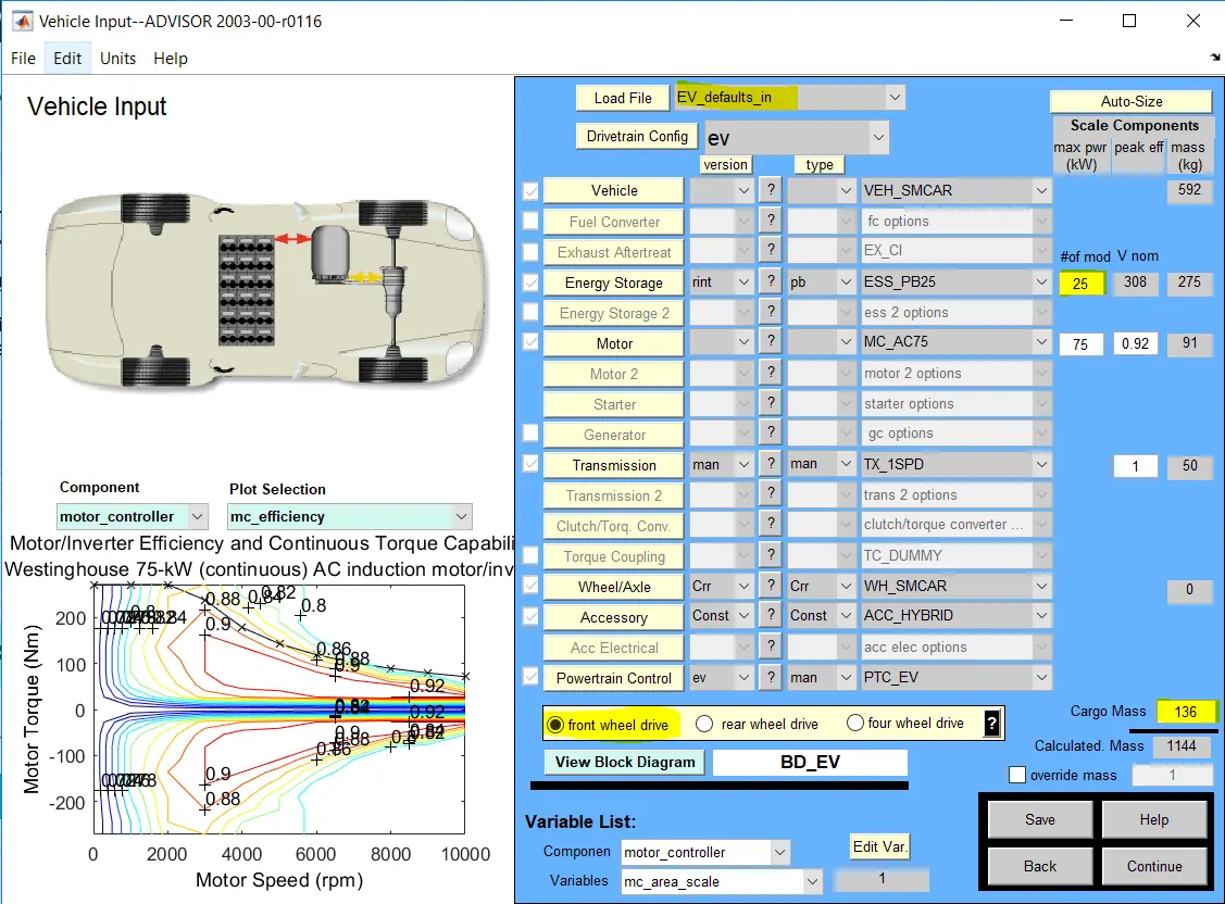
You can see from the image that the Electric vehicle has been updated and I have highlighted some specifications for better understanding. We can see that in the default model there are 25 packs used and the default cargo mass is 136 which we will be increasing to 500kg and we will be using a front-wheel drive.

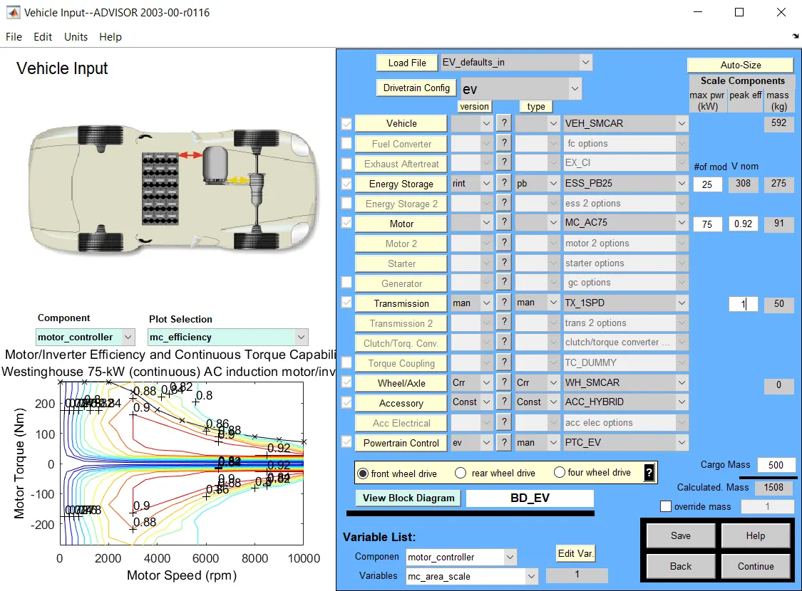
Once the cargo weight is increased the vehicle weight is also updated. After this step, we can click on Continue.

Once we click to continue the Simulation Parameters block will open in which we can update the Drive cycle and various parameters we need to run the simulation.

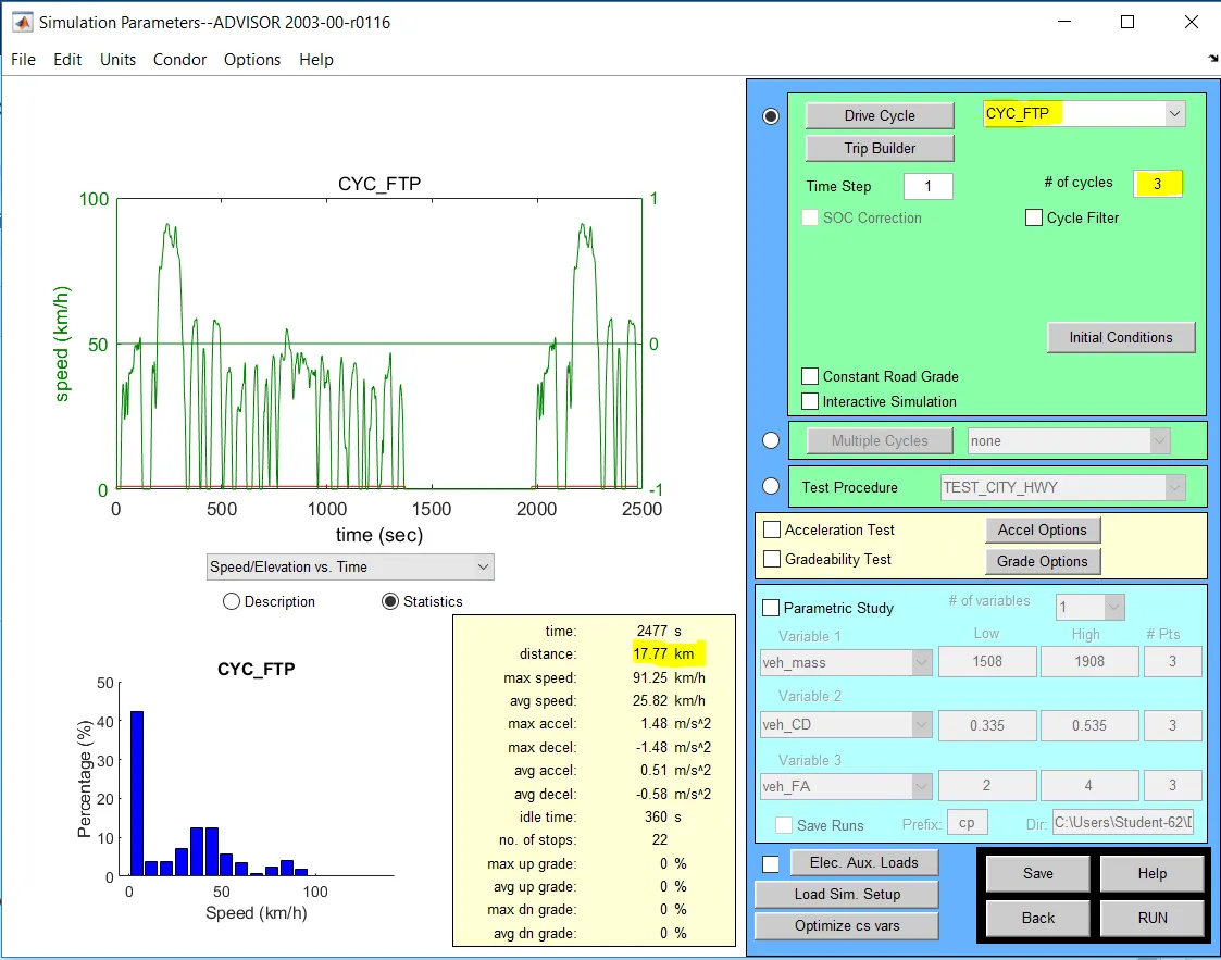
In the above image, you can see that the FTP cycle has been updated and the cycle input we have given as 3. The Distance for one cycle is 17.77 km and if we run 3 times the distance traveled will be 53.31km. The time taken to complete a single cycle is 2477 seconds.

Once the parameters are provided we can click on RUN.

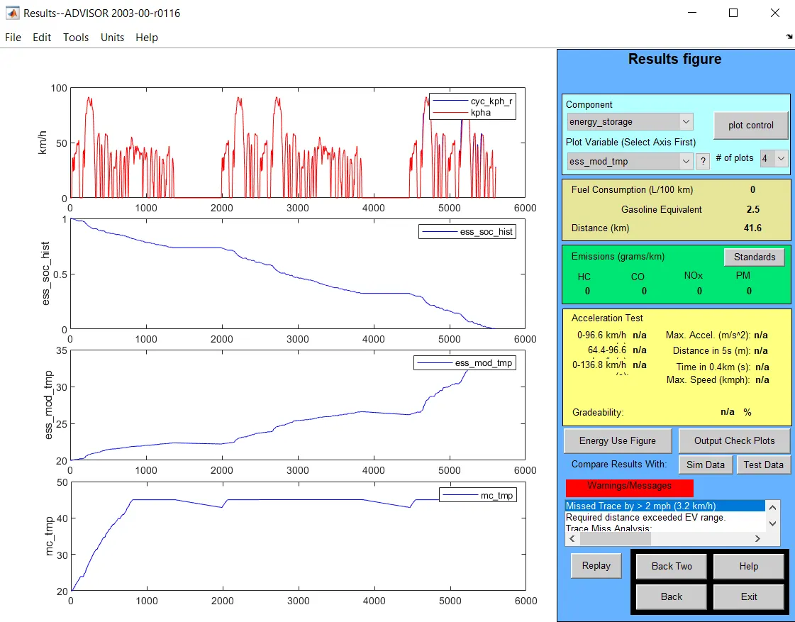
Once we run we can see the above results. We can see from the Second graph that the battery is fully depleted at 41.6 km. So yes with the given capacity of the battery and load the vehicle won't be able to cover a distance of 45km.

The Third graph is between the Average temperature of the battery module. We can see that the temperature increases to about 35 degrees before the battery is fully discharged.

The fourth graph is between the average temperature of the motor and controller. We can see that the temperature is gradually increasing and becomes constant at 45degree.

Objective-2:

As the battery capacity of 25 packs is not enough we will be increasing the battery capacity and running the simulation keeping all the other parameters constant.

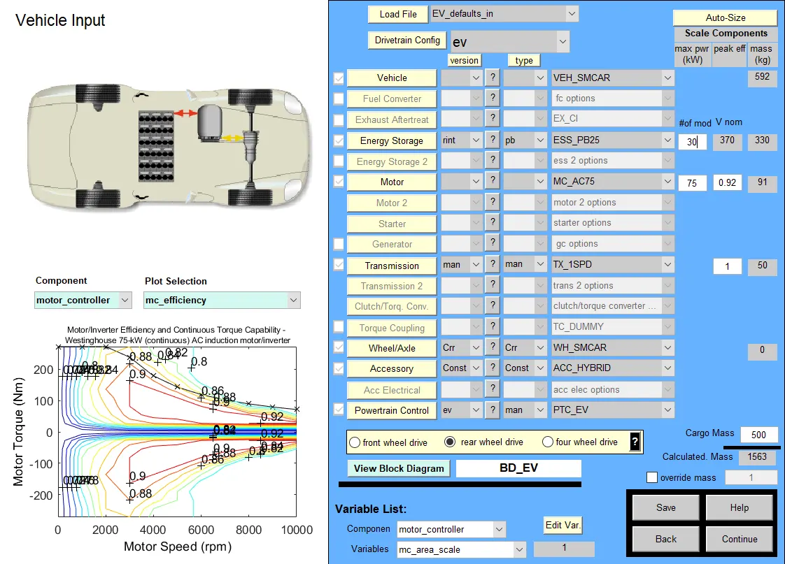
As we increase the pack size to 30 the weight increases and the total weight becomes 1563 kgs.

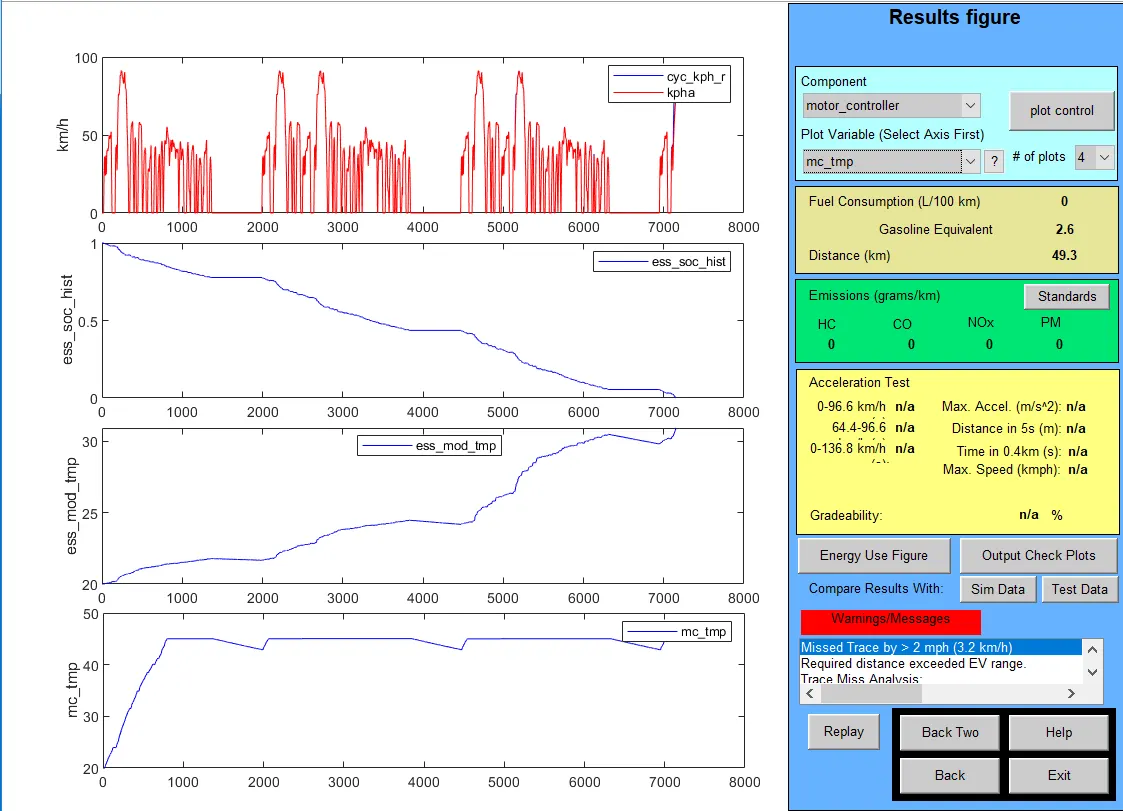
As the battery packs are increased the vehicle is able to cover 45km but the range for 30 packs is 49.3km. As the battery is fully discharged at 49.3 km.

The Third graph is between the Average temperature of the battery module. We can see that the temperature increases to about 30 degrees before the battery is fully discharged.

The fourth graph is between the average temperature of the motor and controller. We can see that the temperature is gradually increasing and becomes constant at 45degree.

Objective-3:

We need to perform a Gradability test for a PRIUS_Jpn_defaults_in file. So first we need to load the file PRIUS_Jpn_defaults_in file in the Vehicle window.

The grade test routine in ADVISOR will determine the maximum grade on which the vehicle can sustain the specified constant speed. The test routine can be accessed both from the GUI and the Matlab command window.

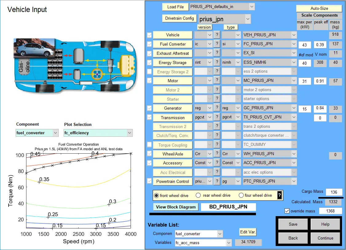
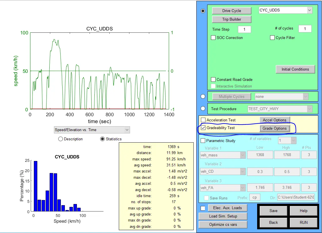
So once we check the gradability check box in the Simulation parameter window. The Grade test Advanced options will open.

Here we will be providing the Grade test parameters.

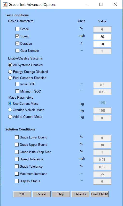
By default, the energy storage system is disabled for the grade test. This option allows us to use a much shorter cycle to determine grade ability based on engine performance alone. This is may not represent reality and thus the ability to enable all systems and to specify an initial and a minimum SOC for the battery pack has been provided.

So for the speed of 30,35,40,45 and 50 mph for a duration of 10 seconds, we will be finding the grade.

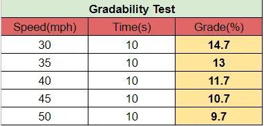
From the above table, you can see that as the Speed increases the Grade percentage decreases.

We can try the same test with the same speed for a duration of 20 seconds.

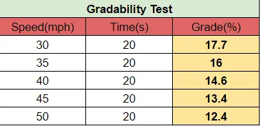
We can see that as time is increased for the above-mentioned speeds the Grade percentage is also increased.

Conclusion:

We have done some basic simulations for various vehicles using the Advisor tool and provided the results with an explanation.