Week-3 Challenge: ADVISOR Tool

AIM:

By using the ADVISOR tool, we need to simulate the given conditions in MATLAB

OBJECTIVE:

• Load ‘EV_defaults_in’ file and change the cargo mass by keeping all the conditions default with FTP drive cycle and conclude the results.
• By changing the battery capacity and number of drive cycles observe the results.
• Load ‘PRIUS_jpn_defaults_in’ file and perform gradeability test and compare the results in table

THEORY:

ADVISOR tool was preliminarily written and used in November 1994 by National Renewable Energy Laboratory (NREL). Since then, it has been modified as necessary to help manage the US DOE Hybrid Vehicle Propulsion System subcontracts. Only in January 1998 was a concerted development effort undertaken to clean up and document ADVISOR.

ADVISOR (ADvanced VehIcle SimulatOR) is a set of model, data, and script text files for use with MATLAB and Simulink. It is designed for rapid analysis of the performance and fuel economy of conventional, electric, and hybrid vehicles. ADVISOR also provides a backbone for the detailed simulation and analysis of user defined drivetrain components, a starting point of verified vehicle data and algorithms from which to take full advantage of the modelling flexibility of Simulink and analytic power of MATLAB.

Benefits of ADVISOR tool:

• It Estimates the fuel economy of vehicles that have not yet been built
• We can learn about how conventional, hybrid, or electric vehicles use (and lose) energy throughout their drivetrains
• It compares relative tailpipe emissions produced on a number of cycles
• Evaluate an energy management strategy for your hybrid vehicle’s fuel converter
• Optimize the gear ratios in your transmission to minimize fuel use or maximize performance, etc.

Limitations:

• Primarily for analysis only, not for design.
• Drive axle is single axle only.

How to run the ADVISOR tool:

• First, download the ADVISOR tool files and extract them in separate folder
• Add the extracted path in MATLAB
• In command window type ‘advisor’ press enter, the ADVISOR interface will appear and select the units as ‘metric’ click on the start
• Another graphical user interface (GUI) – Vehicle parameters window will appear and load the selected file where it will show all the parameters and vehicle layout and plots.
• Click on the continue button, another GUI – Simulation window will open, we have to select drive cycle and number of cycles to run the simulation if needed select acceleration and gradeability test etc.
• Click on the run button, another GUI – Results window will open, where the all the results will be plotted.

1. For EV_defaults_in file, if cargo mass is 500 kg with all other default conditions, can the vehicle travel for 45 km with FTP drive cycle? Conclude your observations.

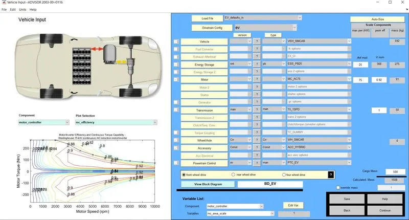
After clicking the start button, now load the EV_defaults_in’ file and change the cargo weight to 500 kg as mentioned. We can notice the change in Calculated mass too. Click on the continue button, simulation window will open.

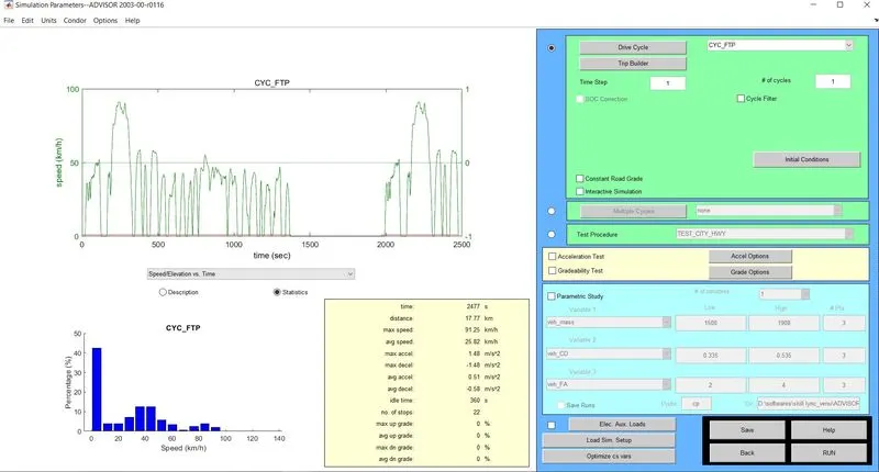
Now, select the drive cycle data file as ‘CYC_FTP’- Federal Test Procedure

We need to run the simulation till the State of Charge (SOC) is completed i.e., 100%

Running the simulation with 1 drive cycle:

Output:

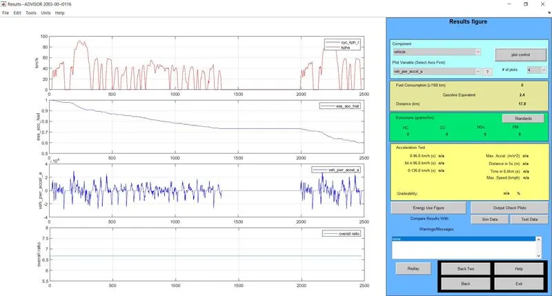
We can observe that the simulation is run for 2500 seconds and distance travelled by the vehicle is 17.8 km.

The SOC value 1 means 100% charged, While the start of the cycle the SOC is ‘1’ at the end SOC is ‘0.6’ means, only 40% on the energy was utilized by the vehicle for 1 drive cycle.

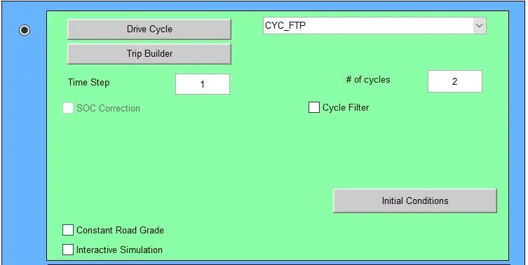
Running the simulation with 2 drive cycle:

Output:

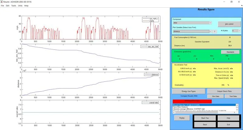
We can observe that the simulation is run for 5000 seconds and distance travelled by the vehicle is 35.5 km.

While the start of the cycle the SOC is ‘1’ at the end SOC is ‘0.18’ means, only 82% on the energy was utilized by the vehicle for 2 drive cycles.

Running the simulation with 3 drive cycle:

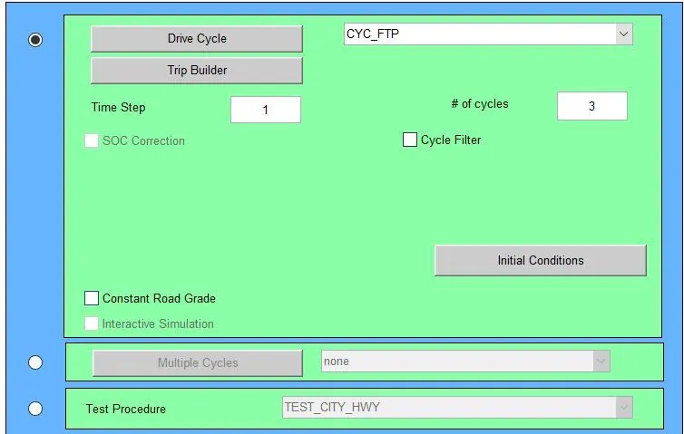
Output:

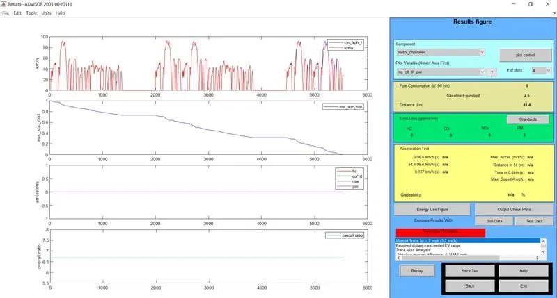
We can observe that the simulation is run for 6000 seconds and distance travelled by the vehicle is 41.4 km.

While the start of the cycle the SOC is ‘1’ at the end SOC is ‘0’ means, 100% on the energy was utilized by the vehicle for 3 drive cycles.

Actual simulation is run for 5500 seconds only because the SOC is ‘0’ i.e., 100% energy utilized by the vehicle.

Number of driving cycles (FTP)	Simulation Time (sec)	Distance travelled (km)	State of Charge Utilized (%)	State of Charge Remained (%)
1	2500	17.8	40	60
2	5000	35.5	82	18
3	6000	41.4	100	0

As pe the condition the vehicle cannot reach the 45 km mark it can reach only 41.4 km with this 3-drive cycle (FTP) because after reaching 41.4 km the SOC is ‘0’.

2. In the above case, try changing the battery capacity and repeat the simulation.

With the same vehicle file, we can change the battery capacity (#of mod) with 2 and 3 drive cycles and observe the results.

a) Energy storage with 25 modules and 2 drive cycle

Output:

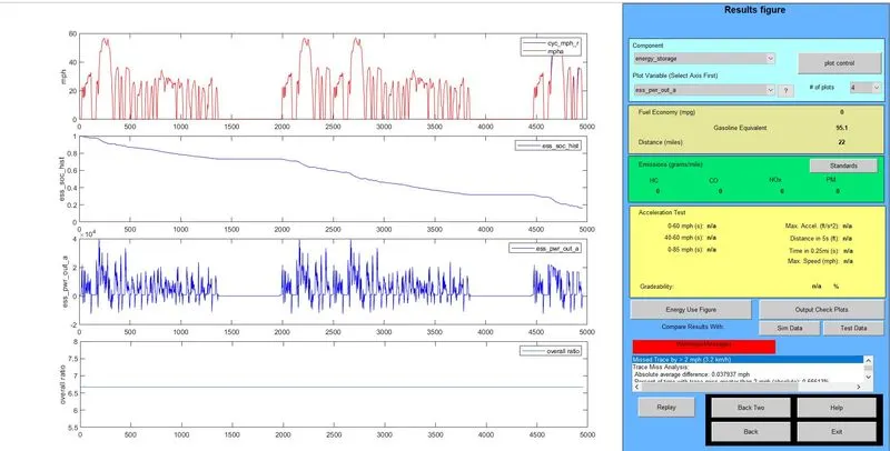
b) Energy storage with 30 modules and 2 drive cycle

Output:

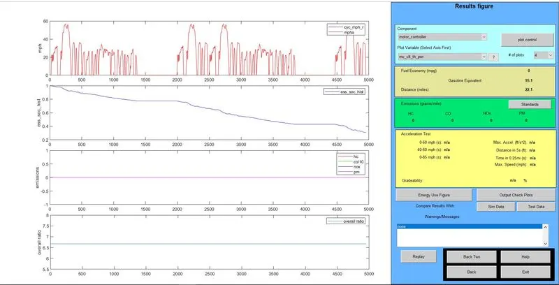
c) Energy storage with 35 modules and 2 drive cycle

Output:

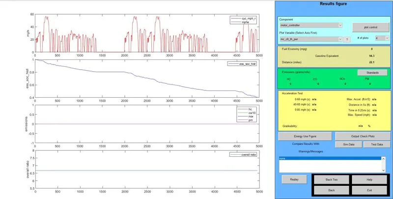
2 Drive cycles
No. of Modules	Voltage	Battery weight (kg)	Distance (miles)	Distance (kmph)
25	308	275	22	35.4
30	370	330	22.1	35.5
35	432	385	22.1	35.5

Here, we can observe that by increasing the number of energy storage modules the distance travelled by the vehicle is almost constant i.e., 35.4 km

d) Energy storage with 25 modules and 3 drive cycle

Output:

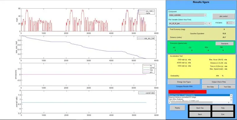
e) Energy storage with 30 modules and 3 drive cycle

Output:

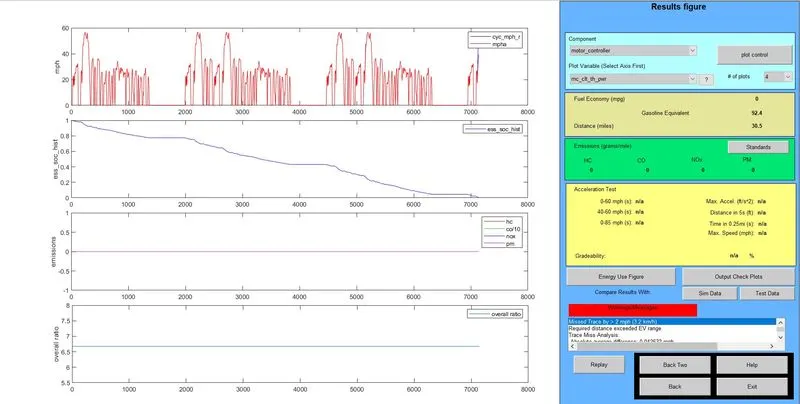
f) Energy storage with 35 modules and 3 drive cycle

Output:

3 Drive cycles
No. of Modules	Voltage	Battery weight (kg)	Distance (miles)	Distance (kmph)
25	308	275	25.7	41.4
30	370	330	30.5	49
35	432	385	33.1	53.3

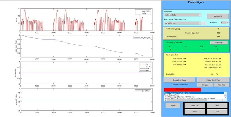
Here, we can observe that by increasing the number of energy storage modules the distance travelled by the vehicle is increasing.

If we want to cover a distance of 50 km then choose the 35 modules and 432 voltage battery which weights 385 kg.

3. Perform gradeability test with PRIUS_Jpn_defaults_in file. Compare your results in table and conclude.

After open the ADVISOR GUI, load the file ‘PRIUS_defaults_in’

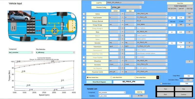
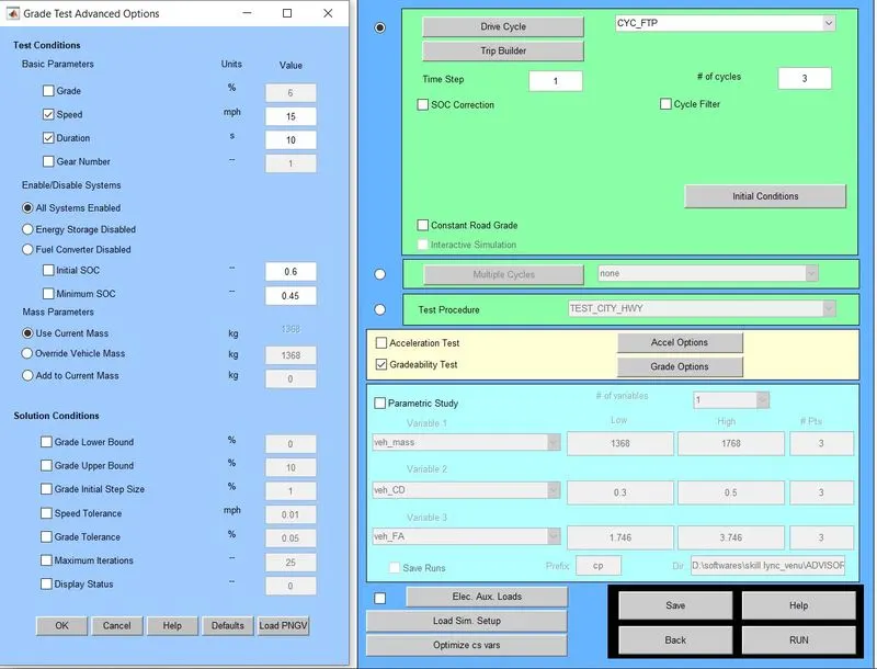
Press the continue button, Simulation setup window will open, in that check the Gradeability Test and click on the Grade options.

The speed and time boxes are checked by default and click on the ‘All Systems Enabled’ button.

Now we need to change the Speed and time so, the gradeability percentage change value can be known.

a) Speed is 15 mph and Duration 10 seconds

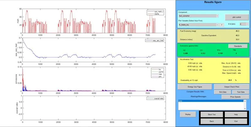
Output:

Gradeability is 24.4%

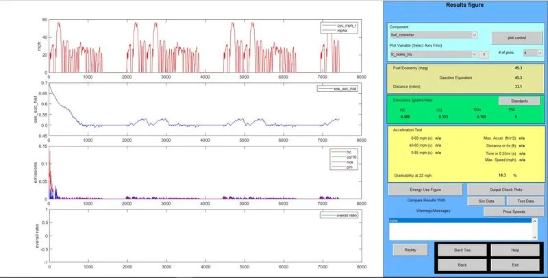
b) Speed is 22 mph and Duration 10 seconds

Output:

Gradeability is 18.3%

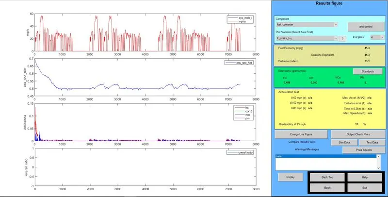
c) Speed is 29 mph and Duration 10 seconds

Output:

Gradeability is 15%

Time Duration 10 seconds
Speed (mph)	Speed (kmph)	Gradeability (%)	Distance (miles)
15	24.1	24.4	31.1
22	35.4	18.3	31.1
29	46.7	15	31.1

d) Speed is 15 mph and Duration 15 seconds

Output:

Gradeability is 27%

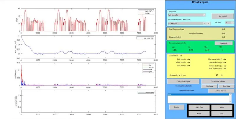
e) Speed is 22 mph and Duration 15 seconds

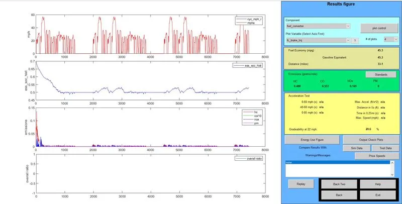
Output:

Gradeability is 20.6%

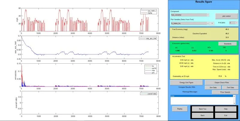
f) Speed is 29 mph and Duration 15 seconds

Output:

Gradeability is 17.2%

Time Duration 20 seconds
Speed (mph)	Speed (kmph)	Gradeability (%)	Distance (miles)
15	24.1	27	31.1
22	35.4	20.6	31.1
29	46.7	17.2	31.1

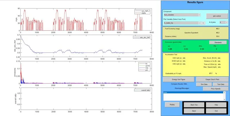
g) Speed is 15 mph and Duration 20 seconds

Output:

Gradeability is 27.7%

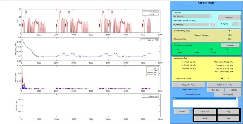
h) Speed is 22 mph and Duration 20 seconds

Output:

Gradeability is 21.3%

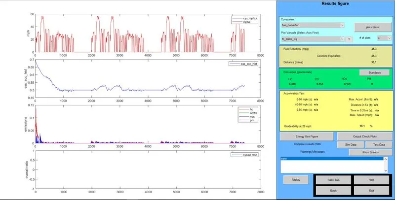
i) Speed is 29 mph and Duration 20 seconds

Output:

Gradeability is 18.1%

Time Duration 30 seconds
Speed (mph)	Speed (kmph)	Gradeability (%)	Distance (miles)
15	24.1	27.7	31.1
22	35.4	21.3	31.1
29	46.7	18.1	31.1

Comparison:

Speed (mph)	Speed (kmph)	Gradeability (%)	Distance (miles)
Time Duration 10 seconds
15	24.1	24.4	31.1
22	35.4	18.3	31.1
29	46.7	15	31.1
Time Duration 20 seconds
15	24.1	27	31.1
22	35.4	20.6	31.1
29	46.7	17.2	31.1
Time Duration 30 seconds
15	24.1	27.7	31.1
22	35.4	21.3	31.1
29	46.7	18.1	31.1

By observing the results, we can conclude that when there is increase in the speed with respect to time the percentage of gradeability decreases and the distance travelled in constant i.e., 31.1 miles.

CONCLUSION:

Hence, we have simulated the given condition in MATLAB with the help of ADVISOR tool.

• After 3 drive cycles (CYC_FTP) the vehicle had run for 41.4 km only.
• By increasing the number of energy storage modules, the distance travelled by the vehicle is increasing along with the weight.
• When increase in the speed with respect to time the percentage of gradeability decreases and the distance travelled in constant.