Week-3 Challenge: ADVISOR Tool
Before Staring I would like to give a short Introduction of Advisor Tool used in Matlab:
-Advanced Vehicle Simulator (ADVISOR) was first developed in November 1994 at the National Renewable Energy Laboratory. It was designed as an analysis tool to assist the US Department of Energy (DOE) in developing technologies for hybrid electric vehicles (HEV) through the Hybrid Electric Vehicle Propulsion System contracts with Ford, General Motors, and DaimlerChrysler. Its primary role is to highlight the system-level interactions of hybrid and electric vehicle components and their impacts on the vehicle performance and fuel economy.
-ADVISOR was created in the MATLAB/Simulink environment. MATLAB provides an easy-to-use matrix-based programming environment for performing calculations while Simulink can be used to represent complex systems graphically using block diagrams. ADVISOR uses three primary graphical user interface (GUI) screens to guide the user through the simulation
process. With the GUIs, the user can iteratively evaluate the impacts of vehicle parameters and drive cycle requirements on the vehicle performance, fuel economy, and emissions.
Intuitive, easy-to-use graphical interface;
Fast solutions;
Distributed as open source code;
Customizable;
Scalable component models;
Good customer support, software maintenance, and documentation;
Free and publicly available;
Highly parameterized models;
Provides robust solutions;
Modular architecture.
- Some of the Advantages of Advisor Tool :
1. To estimate the fuel economy of vehicles that have not been built.
2. We can also learn about how coventional,hybrid or electric vehicle use(and lose)energy throughtout their drivetrains.
3. We can compare relative tailpipe emissions produced on a number of cycles.
4. We can also change / modify no. of battery modules, change drivetains, change in motor etc and find out the best possible solution to meet our vehicle design and model requirements.
- We, can launch the Advisor Tool in the Matlab Software Window by adding its directory in the Matlab Window.
- We can launch the Advisor Tool form the command window of Matlab by typing 'advisor' and press enter.
- A new window will be launched as shown in the below Fig 1.1
ADVISOR tool have 3 windows:
1. Vehicle Input window
2. Simulation Parameter window
3. Results Window
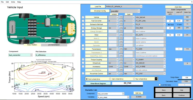
Default Window of Advisor Tool: Fig 1.1
Solution 1. :- For EV_defaults_in file, if cargo mass is 500 kg with all other default conditions, can the vehicle travel for 45 km with FTP drive cycle? Conclude your observations.
Given Data :-
- We have to perform simulation on EV_defaults_in file & to run in the FTP drive cycle.
- We have to also change the cargo defalut value(136kg) to 500kg.
- We have to observe whether we can run our vehicle for 45km distance with all the default values.
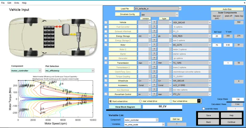
Default Values of EV_defaults_in: Fig 1.2
- As per the given data we have to change the Cargo Value to 500kg so the total weight will be 1508kg
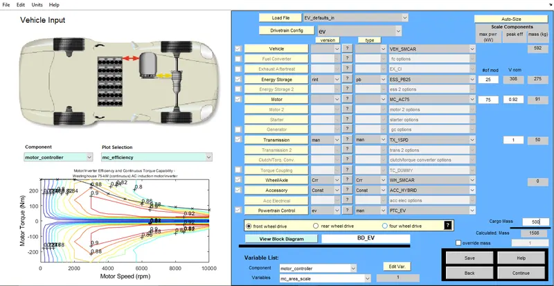
EV_defaults_in Cargo Value @500kg: Fig 1.3
- Now, we have to change the default cycle to CYC_FTP
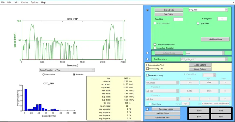
CYC_FTP Selected: Fig 1.4
- We can observe in the output result that for 1 cycle the total distance covered around 17.8km and the used Battery SOC is 40%
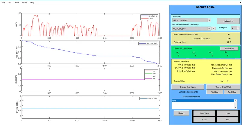
Output Result for 1 Driving CYC_FTP: Fig 1.5
- As, we have to observe whether the vehicle can travel 45km from remaining Battery SOC, so we wil RUN the simulation till the Battery SOC is zero.
- Now, we have add one more CYC_FTP so the # of cycles = 2
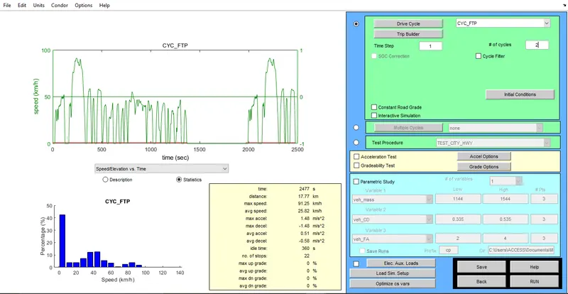
CYC_FTP @2 Cycles: Fig 1.6
- We can observe in the output result that for 2 cycle the total distance covered around 35.5km and the used Battery SOC is 80%
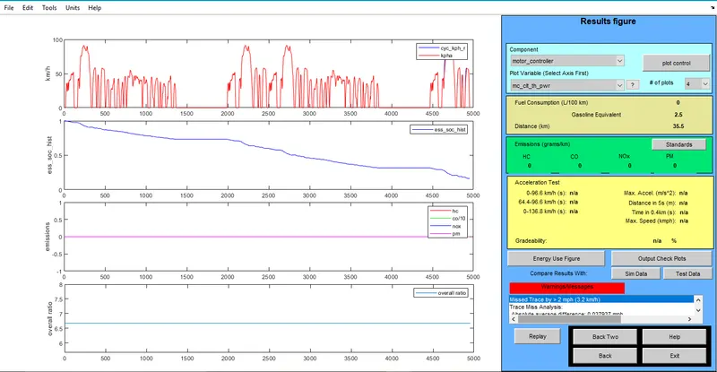
Output Result for 2 Driving CYC_FTP: Fig 1.7
- Now, we have add one more CYC_FTP so the # of cycles = 3
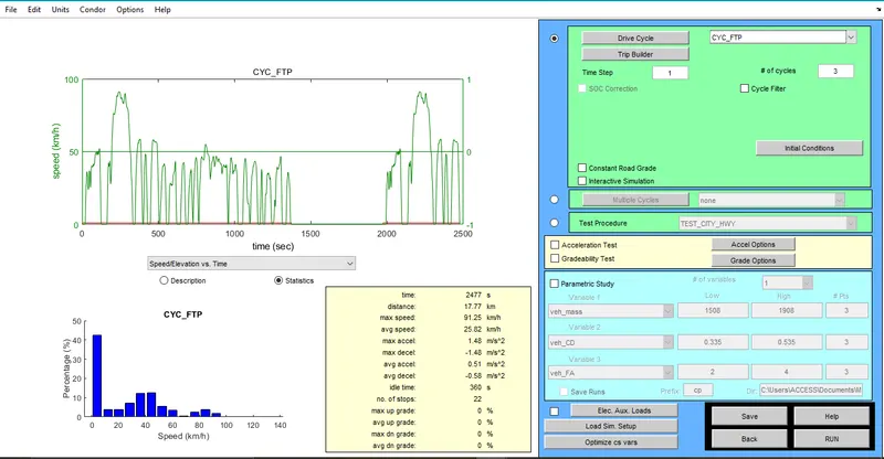
CYC_FTP @3 Cycles: Fig 1.8
- We can observe in the output result that for 3 cycle the total distance covered around 41.4km and the used Battery SOC is 100%
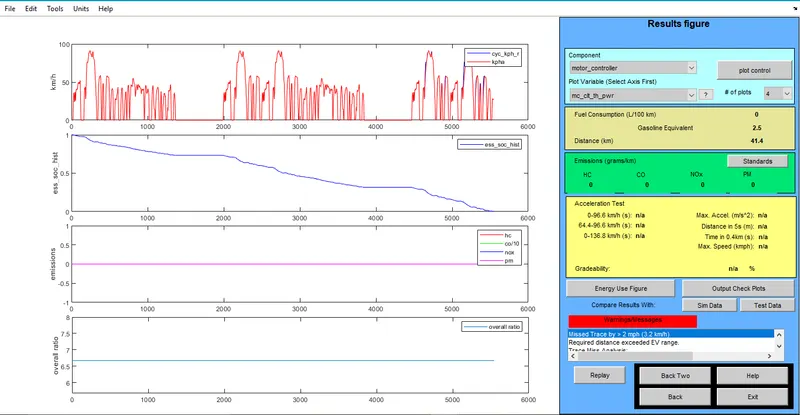
Output Result for 3 Driving CYC_FTP: Fig 1.9
| SR.NO | NUMBER OF DRIVING CYCLES | DISTANCE COVERED(km) | BATTERY SOC(%) |
| 1 | 1 | 17.8 | 40 |
| 2 | 2 | 35.5 | 80 |
| 3 | 3 | 41.4 | 100 |
Conclusion :
- We can observe that after completing our simulation that the minimum distance travelled in the CYC_FTP in 1 cycle is 17.8km, whereas the maximum distance travelled is 41.4km when the Battery SOC 100%.
- Hence, we can conclude that the EV_default_in cannot travel 45km distance due to insufficient Battery SOC.
Solution 2. :- In the above case, try changing the battery capacity and repeat the simulation.
Given Data :
- As, mentioned in the question itself we have to considered the same input parameter to achieve the distance of 45km but in addition we have to make changes in the battery capacity.
- To keep our simulation simple, we are going to increase the no of #of mod by keeping the driving CYC_FTP = 3
- Now, we have add 1 #of mod i.e. 25 >> 26 we can also observe the V nom value changing from 308 >> 321 whereas, the weight increase from 275 >> 286.

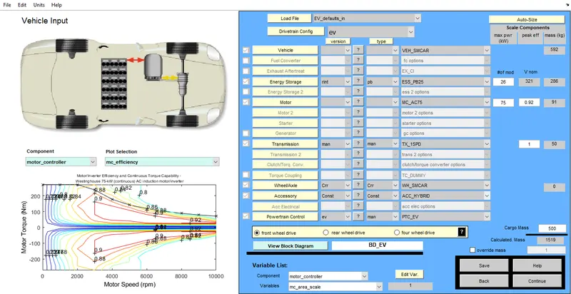
Input Parameter #of mod 25 >> 26: Fig 2.1
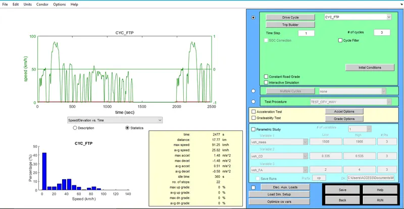
CYC_FTP = 3 Fig 2.2
- As, we can observe in the below mentioned Output result the distance travelled is 42.7km
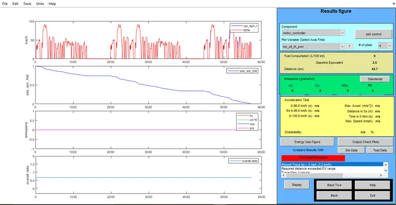
Output Result Distance @42.7km: Fig 2.3
- Now, we have add 1 #of mod i.e. 26 >> 27 we can also observe the V nom value changing from 321 >> 333 whereas, the weight increase from 286 >> 297.

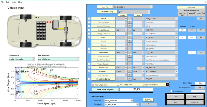
Input Parameter #of mod 26 >> 27: Fig 2.4
- As, we can observe in the below mentioned Output result the distance travelled is 44.8km
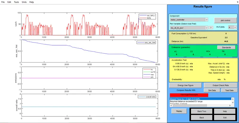
Output Result Distance @44.8km: Fig 2.5
- Now, we have add 1 #of mod i.e. 27 >> 28 we can also observe the V nom value changing from 333 >> 345 whereas, the weight increase from 297 >> 308.

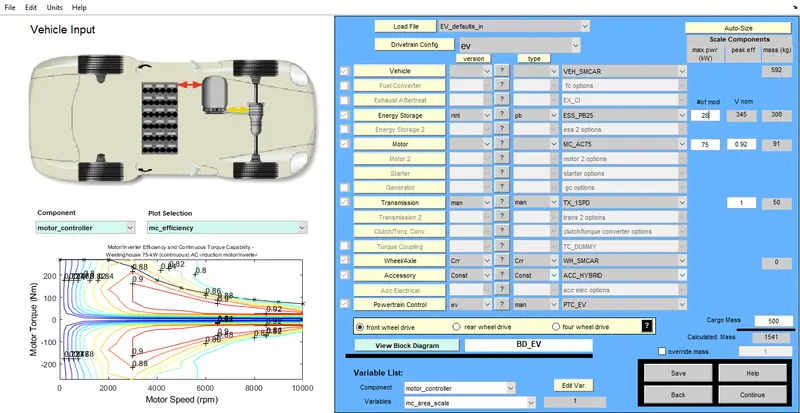
Input Parameter #of mod 27 >> 28: Fig 2.6
- As, we can observe in the below mentioned Output result the distance travelled is 46.3km
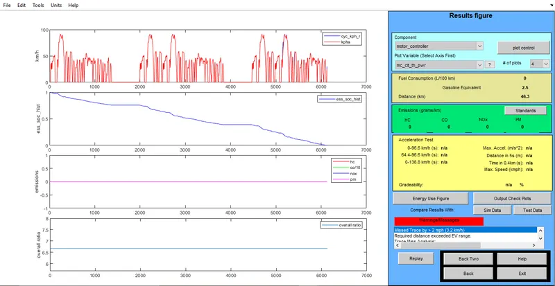
Output Result Distance @46.3km: Fig 2.7
No of Driving Cycles : 03 cycles
| BATTERY MODULES | VOLTAGES | DISTANCE COVERED(km) | BATTERY WEIGHT(kg) |
| 26 | 321 | 42.7 | 286 |
| 27 | 333 | 44.8 | 297 |
| 28 | 345 | 46.3 | 308 |
- From all the above simulation carried by performing the changes in Battery Modules in a step wise we observe that the EV_default_in when there are 28 #of mod we get the vehicle covering the distance of 46.3km. This was the simulation results we were looking for.
- Hence the vehicle to cover the distance of 45km requires 28 no of battery modules and 345-volt battery is required.
Solution 3. :- Perform gradeability test with PRIUS_Jpn_defaults_in file. Compare your results in table and conclude.
Given Data :
- Vehicle to be considered is PRIUS_Jpn_defaults_in
- We have considered all the default parameter values
- We have considered the CYC_FTP for 3 cycles
- To compare vehicle we have considered two different time cycles '10sec' & '25sec'.
- We have selected PRIUS_Jpn_defaults_in as the vehicle
- To perform the Gradeability test we have to set the values of Speed and Time from Simulation Parameter Window
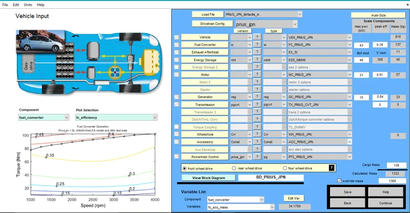
PRIUS_Jpn_defaults_in selected: Fig 3.1
-->> Time Duration = 10 seconds
1. Speed = 20mph or 32.2kmph, Time = 10seconds
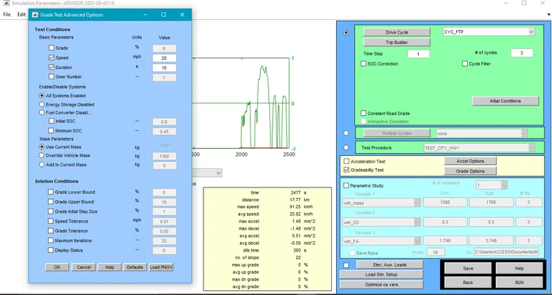
Parameters Set for Speed & Time: Fig 3.2
Output Results : Gradeability : 19.8%
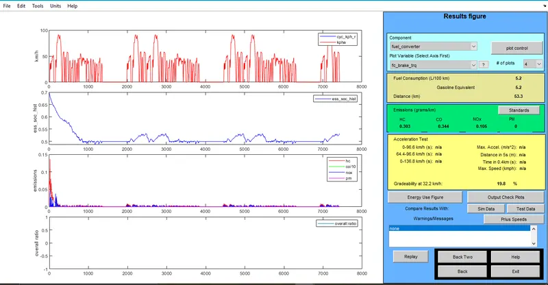
Output Results Gradeability : 19.8% : Fig 3.3
2. Speed = 35mph or 56.3kmph, Time = 10seconds
Output Results : Gradeability : 13%
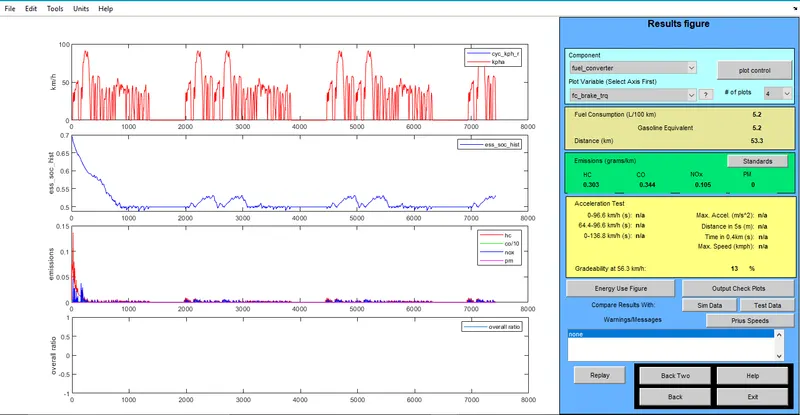
Output Results Gradeability : 13% : Fig 3.4
3. Speed = 50mph or 80.5kmph, Time = 10seconds
Output Results : Gradeability : 9.7%
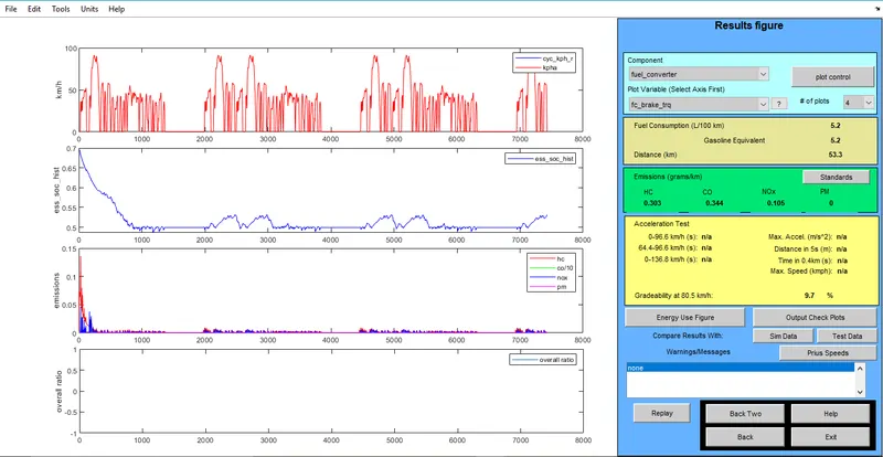
Output Results Gradeability : 9.7% : Fig 3.5
4. Speed = 56.70mph or 91.25kmph, Time = 10seconds
Output Results : Gradeability : 8.6%
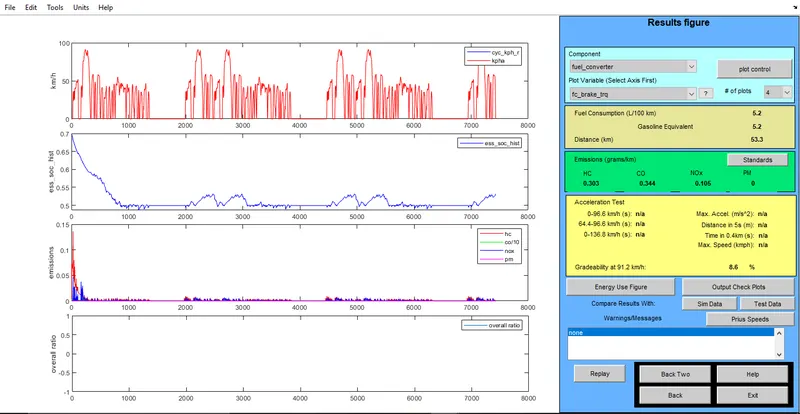
Output Results Gradeability : 8.6% : Fig 3.6
-->> Time Duration = 25 seconds
1. Speed = 20mph or 32.2kmph, Time = 25seconds
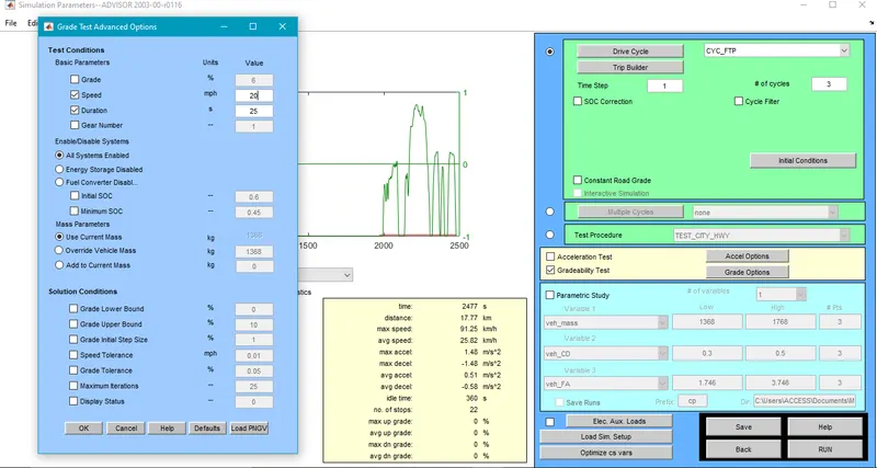
Parameters Set for Speed & Time: Fig 3.7
Output Results : Gradeability : 23.2%
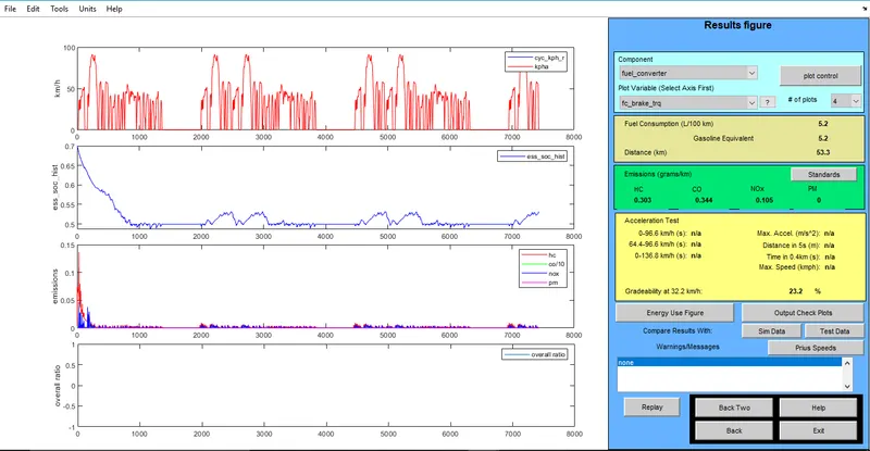
Output Results Gradeability : 23.2% : Fig 3.8
2. Speed = 35mph or 56.3kmph, Time = 25seconds
Output Results : Gradeability : 16.5%
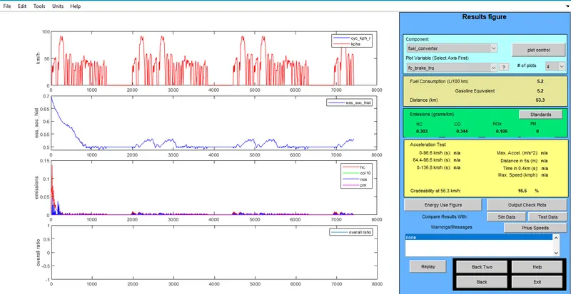
Output Results Gradeability : 16.5% : Fig 3.9
3. Speed = 50mph or 80.5kmph, Time = 25seconds
Output Results : Gradeability : 12.8%
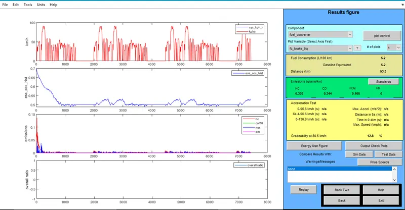
Output Results Gradeability : 12.8% : Fig 3.10
4. Speed = 56.70mph or 91.25kmph, Time = 25seconds
Output Results : Gradeability : 11.6%
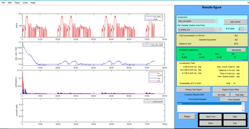
Output Results Gradeability : 11.6% : Fig 3.17
For Time Duration --->>> 10seconds
| SR.NO | VEHICLE SPEED(mph) | VEHICLE SPEED(kmph) | GRADEABILITY(%) |
| 01 | 20 | 32.2 | 19.8% |
| 02 | 35 | 56.3 | 16.5% |
| 03 | 50 | 80.5 | 9.7% |
| 04 | 56.70 | 91.25 | 8.6% |
For Time Duration --->>> 25seconds
| SR.NO | VEHICLE SPEED(mph) | VEHICLE SPEED(kmph) | GRADEABILITY(%) |
| 01 | 20 | 32.2 | 23.2% |
| 02 | 35 | 56.3 | 13% |
| 03 | 50 | 80.5 | 12.8% |
| 04 | 56.70 | 91.25 | 11.6% |
Conclusion :- We, can observe after performing the simulation for time peroid '10seconds' & '25seconds', when the speed of the vehicle increases there is decrease in the Gradeability %.