Week 3 - Adiabatic Flame Temperature calculation
Objective:
- To study the effect of equivalence ratio on Adiabatic flame temperature for methane.
- To study the flame temperature variation with heat loss.
- To study the AFT variation with alkane, alkene, alkyne.
- To study the variation of AFT with no. of carbon atoms in chain.
Adiabatic Flame Temperature
The chemical reaction in which the substance reacts rapidly with oxygen and gives off heat is called combustion. The burning substance is called fuel and the other source is called an oxidizer and fuel can be solid, liquid or gas.
Adiabatic flame temperature is referred to as the maximum amount of heat that is generated when air-fuel mixture is burnt completely without loss of heat.
In the study of combustion, there are two types of Adiabatic flame temperature depending on how the process is completed the constant volume and constant pressure. both of which describe temperature that combustion products theoretically can reach if no energy is lost to the outside environment. The constant volume adiabatic flame temperature is the temperature that results from a complete combustion process that occurs without any work. heat transfer or change in kinetic or potential energy. its temperature is higher than the constant pressure process because no energy is utilized to change the volume of the system.
Theoretically it can be calculated by taking out the difference between the enthalpies of the reactants and products. the enthalpies of substances can be calculated using the polynomial function provided by NASA for a particular temperature.
`h(t) = [a_1+a_2*(T/2)+a_3*(T^2/3)+a_4*(T^3/4)+a_5*(T^4/5)+a_6*(T/6)]*RT`
where, h = enthalpy
`a_i`= coefficients of each species (http://combustion.berkeley.edu/gri-mech/version30/files30/thermo30.dat)
T = temperature
R = gas constant
Coefficients are classified into high temperature coefficients and low temperature coefficients. here, the Newton Raphson scheme is used to solve the enthalpy because it is polynomial function using this method, we will find out the roots of the function using the initial guess and iterate till we reach the given tolerance value. it is defined as
`T_text(new) = T_text(guess)-alpha*[f(T_text(guess))/f^'(T_text(guess))]`
where, `T_text(new)` = new T value after iteration.
`T_text(guess)` = guess value
`alpha` = relaxation factor
Case: 1 Adiabatic flame temperature variation with equivalence ratio (in constant volume chamber)
Equivalence ratio(`phi`) can be defined as the actual air fuel ratio to the stoichiometric air fuel ratio.
if `phi`=1 stoichiometric combustion.
`phi`< 1 lean combustion (Excess air).
`phi`> 1 rich combustion (Excess fuel).
the stoichiometric combustion of the methane is given below.
Stoichiometric mixture
`CH_4 + 2(O_2 + 3.76N_2) -> CO_2 + 2H_2O + 7.52N_2`
lean mixture
`CH_4 + (2/phi)(O_2 + 3.76N_2) -> CO_2 + 2H_2O + (7.52/phi)N2 + (2/phi-2)O_2`
rich mixture
`CH_4 + (2/phi)(O_2 + 3.76N_2) -> (4/phi-3)CO_2 + 2H_2O + (7.52/phi)N_2 + (4-4/phi)CO`
We know that the reactions will be taking place under constant pressure.
Enthalpy balance equation will be as follows:
`h_text(product)-h_text(reactant) -R(n_text(product)*T-n_text(reactant)*T_text(std))`
The relaxation factor is taken as 0.2 and it can be increased up to 0.9 and the behavior change of the solution can be verified. Further, if we increase the relaxation factor above 1 the solution may overshoot and diverge.
Program with explanation
"""
in this program we are going to calculate the AFT of Methane
at different equivalence ratio
Stoitiometric mixture
CH4 + 2(O2 + 3.76N2) = CO2 + 2H2O + 7.52N2
lean mixture
CH4 + 2.5(O2 + 3.76N2) = CO2 + 2H2O + 9.4N2 + 0.5O2
rich mixture
CH4 + 2/(1.2)(O2 + 3.76N2) = ((4/1.2)-3)CO2 + 2H2O + (7.52/1.2)N2 + (4-(4/1.2))CO

"""
import matplotlib.pyplot as plt
import cantera as ct
import math
import numpy as np
R = 8.314    #Gas constant(j/mol-K)
def h(T,co_effs):
	"""
		function to evaluate enthalpy
	"""

	T_std = 298.15


	a1 = co_effs[0]
	a2 = co_effs[1]
	a3 = co_effs[2]
	a4 = co_effs[3]
	a5 = co_effs[4]
	a6 = co_effs[5]

	return (a1 + a2*T/2 + a3*pow(T,2)/3 + a4*pow(T,3)/4 + a5*pow(T,4)/5 + a6/T)*R*T


# coefficients of different spesies at different conditions
CH4_coeff_l = [5.14987613E+00, -1.36709788E-02, 4.91800599E-05, -4.84743026E-08, 1.66693956E-11, -1.02466476E+04, -4.64130376E+00]
O2_coeff_l = [3.78245636E+00, -2.99673416E-03, 9.84730201E-06, -9.68129509E-09, 3.24372837E-12, -1.06394356E+03, 3.65767573E+00]
O2_coeff_h = [3.28253784E+00, 1.48308754E-03, -7.57966669E-07, 2.09470555E-10, -2.16717794E-14, -1.08845772E+03, 5.45323129E+00]
N2_coeff_h = [0.02926640E+02, 0.14879768E-02, -0.05684760E-05, 0.10097038E-09, -0.06753351E-13, -0.09227977E+04, 0.05980528E+02]
N2_coeff_l = [0.03298677E+02, 0.14082404E-02, -0.03963222E-04, 0.05641515E-07, -0.02444854E-10, -0.10208999E+04, 0.03950372E+02 ]
CO2_coeff_h = [3.85746029E+00, 4.41437026E-03, -2.21481404E-06, 5.23490188E-10, -4.72084164E-14, -4.87591660E+04, 2.27163806E+00]
H2O_coeff_h = [3.03399249E+00, 2.17691804E-03, -1.64072518E-07, -9.70419870E-11, 1.68200992E-14, -3.00042971E+04, 4.96677010E+00]
CO_coeff_h = [2.71518561E+00, 2.06252743E-03, -9.98825771E-07, 2.30053008E-10, -2.03647716E-14, -1.41518724E+04, 7.81868772E+00]


def f(T, Phi):
	"""
	calculating enthalpies for products and reactants

	"""
	T_std = 298.15

	h_CH4_r = h(T_std,CH4_coeff_l)
	h_O2_r = h(T_std,O2_coeff_l)
	h_N2_r = h(T_std,N2_coeff_l)

	H_reactant = (h_CH4_r + (2/Phi)*h_O2_r + (7.52/Phi)*h_N2_r)
	N_reactant = (1+(2/Phi)) + (7.52/Phi)*R*T_std

	h_CO2_p = h(T,CO2_coeff_h)
	h_N2_p = h(T,N2_coeff_h)
	h_H2O_p = h(T,H2O_coeff_h)
	h_O2_p = h(T,O2_coeff_h)
	h_CO_P = h(T,CO_coeff_h)


	if Phi >= 1:
		H_product = ((4/Phi)-3)*h_CO2_p + 2*h_H2O_p + (7.52/Phi)*h_N2_p + (4-(4/Phi))*h_CO_P
		N_product = ((4/Phi-3) + 2 + (7.52/Phi) + (4-4/Phi))*R*T


	elif Phi < 1:
		H_product = h_CO2_p + 2*h_H2O_p + (7.52/Phi)*h_N2_p + ((2/Phi)-2)*h_O2_p
		N_product = (1 + 2 +( 7.52/Phi) + (2/Phi - 2))*R*T

	return (H_product - H_reactant) - (N_product - N_reactant)


def fprime(T, Phi):
	return (f(T+1e-6,Phi) - f(T,Phi))/(1e-06)


#Defining Newton-Raphson method

alpha = 0.2
tol = 1e-3
Phi = np.linspace(0.5,2,100)
iter = 1
Temp = []
for i in range(0,len(Phi)):
	T_guess = 1500 #K

	while (abs(f(T_guess,Phi[i])) >= tol):
		T_guess = T_guess - alpha*(f(T_guess, Phi[i])/fprime(T_guess, Phi[i]))
		#plt.plot(iter,T_guess,'*',color='red')
		#print(T_guess)
		iter = iter+1
	Temp.append(T_guess)
print('no. of iterations ',iter)
print('maximum adiabatic flame temperature observed in python is ',max(Temp))


"""
code to calculate the AFT using cantera
"""
gas = ct.Solution('gri30.xml')
Temp_ct = []
for i in range(0,len(Phi)):
	n_total = 1+(2/Phi[i]) + (7.52/Phi[i])
	n_CH4 = 1/n_total
	n_O2 = (2/Phi[i])/n_total
	n_N2 = (7.52/Phi[i])/n_total
	gas.TPX = 298.15,101325, {'CH4':n_CH4, 'O2':n_O2, 'N2':n_N2}
	gas.equilibrate('UV','auto')
	Temp_ct.append(gas.T)
print('maximum adiabatic flame temperature observed in cantera is ',max(Temp_ct))


#Plotting
plt.plot(Phi,Temp,'-*',color='red',label='Python')
plt.plot(Phi,Temp_ct,'-*',color='blue',label='Cantera')
plt.xlabel('Equivalence ratio (Phi)', fontsize=14)
plt.ylabel('Adiabatic flame temperature[K]',fontsize=14)
#plt.grid('on')
plt.title('Adiabatic flame temperature VS Equivalance ratio for methane-air combustion', fontsize=16, fontweight='bold')
plt.legend(fontsize=14)
plt.show()
Output plot and results for case 1
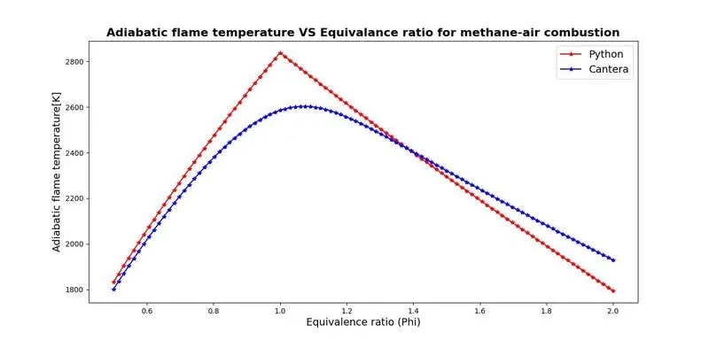

It can be seen that the maximum temperature attained in Cantera is 2603.24K and 2838.23K in python. The decrease in the temperature can be observed as compared to python, this is due to the process through which the Cantera solves, it uses the Gibbs free energy to reach the equilibrium state.
Other than that, many other species are formed in Cantera that are not considered in the python program for different mixtures.
Case: 2 Flame Temperature Variation with heat loss (constant pressure chamber)
Heat loss is considered for this case in the constant pressure chamber; thus, the reaction is not going to be an adiabatic reaction.
the heat loss in the program can be calculated from the lower heating value (LHV). LHV can be obtained from the difference of products and reactants at STP condition.
`LHV = H_(CH_4)^298.18+2H_(O_2)^298.15-H_(CO_2)^298.15+7.52N_2`
The heat loss factor varied from no heat loss to entire heat loss as a multiplier of LHV. further after the heat loss the enthalpy equation changes to:
`H_text(product)-H_text(reactant)+H_text(loss) = 0`
Where, loss = heat loss*LHV
Program with explanation
"""
in this program we are going to calculate the AFT with heat loss at constant pressure for methane

CH4 + 2(O2 + 3.76N2) = CO2 + 2H2O + 7.52N2
"""
import matplotlib.pyplot as plt
import math
import numpy as np


Heat_loss = np.linspace(0,1,50)
def h(T,co_effs):
	"""
		function to evaluate enthalpy
	"""


	R = 8.314    #Gas constant(j/mol-K)

	a1 = co_effs[0]
	a2 = co_effs[1]
	a3 = co_effs[2]
	a4 = co_effs[3]
	a5 = co_effs[4]
	a6 = co_effs[5]

	return (a1 + a2*T/2 + a3*pow(T,2)/3 + a4*pow(T,3)/4 + a5*pow(T,4)/5 + a6/T)*R*T


#low temp coeffs
CH4_coeff_l = [5.14987613E+00, -1.36709788E-02, 4.91800599E-05, -4.84743026E-08, 1.66693956E-11, -1.02466476E+04, -4.64130376E+00]
O2_coeff_l = [3.78245636E+00, -2.99673416E-03, 9.84730201E-06, -9.68129509E-09, 3.24372837E-12, -1.06394356E+03, 3.65767573E+00]
N2_coeff_l = [0.03298677E+02, 0.14082404E-02, -0.03963222E-04, 0.05641515E-07, -0.02444854E-10, -0.10208999E+04, 0.03950372E+02 ]


#high temp coeffs
O2_coeff_h = [3.28253784E+00, 1.48308754E-03, -7.57966669E-07, 2.09470555E-10, -2.16717794E-14, -1.08845772E+03, 5.45323129E+00]
N2_coeff_h = [0.02926640E+02, 0.14879768E-02, -0.05684760E-05, 0.10097038E-09, -0.06753351E-13, -0.09227977E+04, 0.05980528E+02]
CO2_coeff_h = [3.85746029E+00, 4.41437026E-03, -2.21481404E-06, 5.23490188E-10, -4.72084164E-14, -4.87591660E+04, 2.27163806E+00]
H2O_coeff_h = [3.03399249E+00, 2.17691804E-03, -1.64072518E-07, -9.70419870E-11, 1.68200992E-14, -3.00042971E+04, 4.96677010E+00]
CO_coeff_h = [2.71518561E+00, 2.06252743E-03, -9.98825771E-07, 2.30053008E-10, -2.03647716E-14, -1.41518724E+04, 7.81868772E+00]


T_std = 298.15

"""
	computing max possible heat loss
"""
LHV = h(T_std,CH4_coeff_l) + 2*h(T_std,O2_coeff_l)-h(T_std,CO2_coeff_h)-2*h(T_std,H2O_coeff_h)


#computing enthalpies for products and reactants

def f(T, Heat_loss):


	h_CO2_p = h(T,CO2_coeff_h)
	h_N2_p = h(T,N2_coeff_h)
	h_H2O_p = h(T,H2O_coeff_h)


	H_product = h_CO2_p + 2*h_H2O_p + 7.52*h_N2_p

	T_std = 298.15


	h_CH4_r = h(T_std,CH4_coeff_l)
	h_O2_r = h(T_std,O2_coeff_l)
	h_N2_r = h(T_std,N2_coeff_l)

	H_reactant = h_CH4_r + 2*h_O2_r + 7.62*h_N2_r

	return H_product - H_reactant + (Heat_loss*LHV)


def fprime(T, Heat_loss):
	return (f(T+1e-6,Heat_loss) - f(T,Heat_loss))/(1e-06)


#Defining Newton-Raphson method

alpha = 0.8
tol = 1e-3
Temp = []
for i in Heat_loss:
	T_guess = 1500 #K

	while (abs(f(T_guess,i)) > tol):
		T_guess = T_guess - alpha*(f(T_guess, i)/fprime(T_guess, i))
	Temp.append(T_guess)

print(Temp)
Temp_loss = Temp[7]
print(Temp_loss)

#Plotting
plt.plot(Heat_loss,Temp,'*',color='red')
plt.xlabel('heat loss coeff', fontsize=14)
plt.ylabel('Adiabatic flame temperature[K]',fontsize=14)
#plt.grid('on')
plt.title('variation of aft with heat loss', fontsize=16, fontweight='bold')
plt.grid ('on')
plt.show()
Output plot
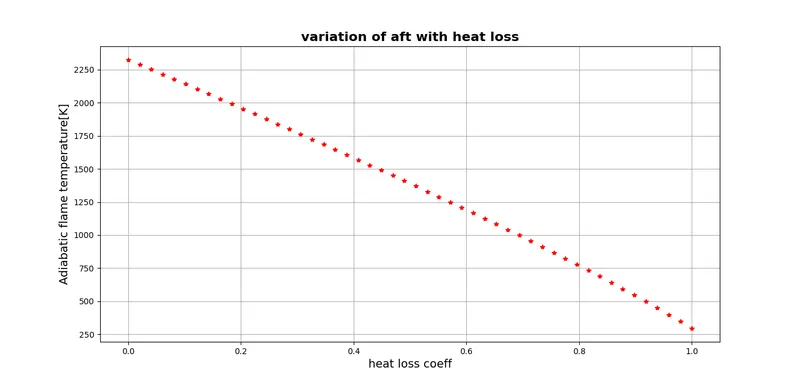
It can be observed from the figure that with an increase in heat loss the temperature of the flame decreases because heat is getting lost from the system.
When the heat loss is zero the flame temperature is 2325K and when the heat loss is 1 the flame temperature drops to 295.95K.
Case: 3 Adiabatic flame temperature variation with respect to alkane, alkene and alkyne.
in this case, we have to consider an alkane, alkene and alkyne for the reaction.
Alkane
`C_2H_6+3.5(O_2+3.76N_2)->2CO_2+3H_2O+13.16N_2`
Alkene
`C_2H_4+3(O_2+3.76N_2)->2CO_2+2H_2O+11.28N_2`
Alkyne
`C_2H_2+2.5(O_2+3.76N_2)->2CO_2+H_2O+9.4N_2`
Program with explanation
import matplotlib.pyplot as plt
import cantera as ct
import numpy as np

gas = ct.Solution('gri30.xml')


#calculating AFT for ethane
gas.TPX = 298.15,101325,{'C2H6':1 ,'O2':3.5, 'N2':13.16}
gas.equilibrate('HP','auto')
T_C2H6 = gas.T


#calculating AFT for ethene

gas.TPX = 298.15,101325,{'C2H4':1 ,'O2':3.5, 'N2':11.28}
gas.equilibrate('HP','auto')
T_C2H4 = gas.T

#calculating AFT for ethyne

gas.TPX = 298.15,101325,{'C2H2':1 ,'O2':3.5, 'N2':9.4}
gas.equilibrate('HP','auto')
T_C2H2 = gas.T

print('AFT for alkane is ',T_C2H6)
print('AFT for alkene is ',T_C2H4)
print('AFT for alkyne is ',T_C2H2)

#plotting
plt.figure()
plt.bar(['ethane','ethene','ethyne'],Temp,color = 'blue')
plt.xlabel('Hydrocarbon Type')
plt.ylabel('Adiabatic Flame Temperature')
plt.title('Hydrocarbon Type vs AFT', fontsize = 16, fontweight = 'bold')
plt.show()
Output plot
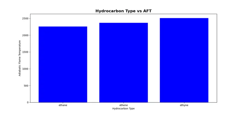
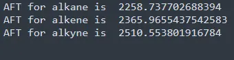
It can be observed that AFT is minimum for the alkane and maximum for the alkyne.
Case: 4 Variation of AFT with respect to variation in number of carbon atoms in chain.
In this case, we will increase the carbon atoms in alkane and observe the change in AFT.
Fuel used will be methane, ethane and propane.
Program with explanation
import matplotlib.pyplot as plt
import math
import numpy as np
import cantera as ct


def h(T,co_effs):
	"""
		function to evaluate enthalpy
	"""


	R = 8.314    #Gas constant(j/mol-K)

	a1 = co_effs[0]
	a2 = co_effs[1]
	a3 = co_effs[2]
	a4 = co_effs[3]
	a5 = co_effs[4]
	a6 = co_effs[5]

	return (a1 + a2*T/2 + a3*pow(T,2)/3 + a4*pow(T,3)/4 + a5*pow(T,4)/5 + a6/T)*R*T


#low temp coeffs
CH4_coeff_l = [5.14987613E+00, -1.36709788E-02, 4.91800599E-05, -4.84743026E-08, 1.66693956E-11, -1.02466476E+04, -4.64130376E+00]
C2H6_coeff_l = [4.29142492E+00, -5.50154270E-03, 5.99438288E-05, -7.08466285E-08, 2.68685771E-11, -1.15222055E+04, 2.66682316E+00]
C3H8_coeff_l = [0.93355381E+00, 0.26424579E-01, 0.61059727E-05, -0.21977499E-07, 0.95149253E-11, -0.13958520E+05, 0.19201691E+02 ]
O2_coeff_l = [3.78245636E+00, -2.99673416E-03, 9.84730201E-06, -9.68129509E-09, 3.24372837E-12, -1.06394356E+03, 3.65767573E+00]
N2_coeff_l = [0.03298677E+02, 0.14082404E-02, -0.03963222E-04, 0.05641515E-07, -0.02444854E-10, -0.10208999E+04, 0.03950372E+02 ]


#high temp coeffs
O2_coeff_h = [3.28253784E+00, 1.48308754E-03, -7.57966669E-07, 2.09470555E-10, -2.16717794E-14, -1.08845772E+03, 5.45323129E+00]
N2_coeff_h = [0.02926640E+02, 0.14879768E-02, -0.05684760E-05, 0.10097038E-09, -0.06753351E-13, -0.09227977E+04, 0.05980528E+02]
CO2_coeff_h = [3.85746029E+00, 4.41437026E-03, -2.21481404E-06, 5.23490188E-10, -4.72084164E-14, -4.87591660E+04, 2.27163806E+00]
H2O_coeff_h = [3.03399249E+00, 2.17691804E-03, -1.64072518E-07, -9.70419870E-11, 1.68200992E-14, -3.00042971E+04, 4.96677010E+00]
CO_coeff_h = [2.71518561E+00, 2.06252743E-03, -9.98825771E-07, 2.30053008E-10, -2.03647716E-14, -1.41518724E+04, 7.81868772E+00]

T_std = 298.15

h_CH4_r = h(T_std,CH4_coeff_l)
h_C2H6_r = h(T_std,C2H6_coeff_l)
h_C3H8_r = h(T_std,C3H8_coeff_l)

c1 = h_CH4_r
c2 = h_C2H6_r
c3 = h_C3H8_r

c = [c1,c2,c3]

#calculating enthalpies for reactants and products
def f(T,c):
	h_CO2_p = h(T,CO2_coeff_h)
	h_N2_p = h(T,N2_coeff_h)
	h_H2O_p = h(T,H2O_coeff_h)

	h_O2_r = h(T_std,O2_coeff_l)
	h_N2_r = h(T_std,N2_coeff_l)


	if c==c1:
		x = 1
		y = 2*(x+1)
		a = x+(y/4)
		b = y/2

		H_product = x*h_CO2_p+b*h_H2O_p+3.76*a*h_N2_p
		H_reactant = c1+a*h_O2_r+(a*3.76)*h_N2_r

	elif c==c2:
		x = 2
		y = 2*(x+1)
		a = x+(y/4)
		b = y/2


		H_product = x*h_CO2_p+b*h_H2O_p+3.76*a*h_N2_p
		H_reactant = c2+a*h_O2_r+(a*3.76)*h_N2_r

	elif c==c3:
		x = 3
		y = 2*(x+1)
		a = x+(y/4)
		b = y/2


		H_product = x*h_CO2_p+b*h_H2O_p+a*3.76*h_N2_p
		H_reactant = c3+a*h_O2_r+(a*3.76)*h_N2_r

	return (H_product - H_reactant)

def fprime(T,c):
	return (f(T+1e-6,c)-f(T,c))/1e-6


#Defining Newton-Raphson method

tol = 1e-3
alpha = 0.2
Temp = []
T_guess = 1500

for i in c:
	T_guess = 1500
	R = 8.314
	while (abs(f(T_guess,i))>tol):
		T_guess = T_guess - alpha*(f(T_guess, i)/fprime(T_guess, i))

	Temp.append(T_guess)

print(Temp)


#Plotting
plt.figure()
plt.bar(['Methane','Ethane','Propane'],Temp)
plt.ylabel('Adiabatic flame temperature [K]')
plt.title('AFT for different no. of carbon atoms in hydrocarbon')
plt.show()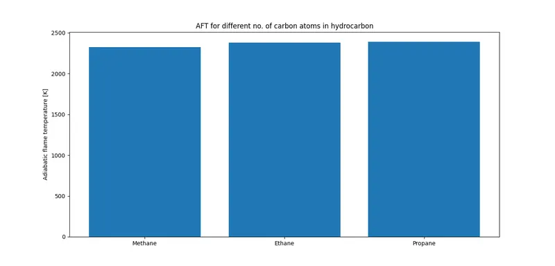
It can be observed that the temperature increases in ascending order from the methane to propane. This could be due to an increase in no. of carbon atoms and hydrogen atoms in the chain.
The temperatures of the hydrocarbons are
Methane: 2325.598K
Ethane: 2379.85K
Propane: 2392.09K
Conclusion
- The maximum flame temperature for a mixture is achieved in the case of a stoichiometric mixture. for rich and lean mixture of the flame temperatures are always less than that of the stoichiometric mixture.
- We used two approaches here (python and Cantera) and there is a difference in results of Cantera and python, this is because Cantera solves by reducing the Gibbs free energy of the equation. Also, it produces more intermediate byproducts for the reaction mechanism than we produce manually.
- If there is a heat loss then we also get a decrease in the Flame temperature.