Week 3 - Adiabatic Flame Temperature calculation
Assignment no. 1
Assignment name- Adiabatic Flame Temperature (python and cantera)
Objective of this assignment-
Case 1- Determine effect of equivalence ratio on AFT in a constant volume chamber for methane.
Write the program in python and compare with cantera
Case 2-To calculate the AFT for methane combustion with heat loss in a constant pressure chamber
Case 3- Adiabatic flame temperature variation with respect to Alkane, Alkene, Alkyne
Case 4- Adiabatic flame temperature variation with respect to number of Carbon atom chains
Theory and introductions
Adiabatic Flame temperature-
- Final temperature obtained after the fuel is completely burned called as adiabatic flame temperature
- When the combustion is takes place energy is released to the combustion product. If no heat loss in this process, the temperature of combustion product is known as adiabatic flame temperature
- There are two types of Adiabatic flame temperature depending upon how is process completed i.e. constant volume/constant pressure
Significance-
- It is characteristics the quality of fuel
- It is used for determine which fuel is suitable for particular application
- The adiabatic flame temperature is very important in design and scale up procedures where heat transfer is significant consideration
Some important concept
Stoichiometric combustion-
- It is a theoretical position in which the optimal amount of oxygen and fuel mix generates the most heat possible, achieving maximum combustion efficiency. There is no unburnt combustibles and no excess air. It is something to strive for, though in reality it does not exits
- In stoichiometry is founded on the law of conservation of mass where the total mass of the reactants equals to total mass of products.
Lean combustion-
- If the amount of air is more than required for complete combustion, there will be excess air after combustion
Rich combustion
- If the amount of air is less than required for complete combustion, part of the fuel would not be fully oxidized such that either will be excess fuel after combustion
Equivalence ratio-
- The fuel air equivalence ratio, (phi), of a system is defined as the ratio of the fuel to oxidizer ratio to the stoichiometric fuel to oxidizer ratio
General equations
CxHy +(x+y/4)(O2+3.76N2)=xCO2 +y/2H2O +(x+y/4)3.76N2
Chemical reaction pf methane
Stoichiometric combustion
CH4+2(O2+3.76N2) =CO2 +2H2O +7.52N2
Lean combustion
CH4 +2/phi(O2+3.76N2) =CO2 +2H2O +7.52/phi N2+(2/phi-2) O2
Rich combustion
CH4 +2/phi(O2+3.76N2) = (4/phi -3) CO2 +2H2O +7.52/phi N2+(4-4/phi) CO
Constant volume process
For constant volume process internal energy is equated for reactants and product to get the AFT
Ur-Up=0
After we will used newton Rapson method and we get final temperature
(H_product-n_prod*R*T)-(Hreactant-N-reactants-n_react*R*Tstd)=0
Coding approach-
1.enthalpy of product and reactants calculated from formula that means nasa polynomial
2.coefficient a1-a7 is directly obtained from Berkeley website
3.For the constant volume method process internal energy is equated for reactants and product to get the AFT
Ur-Up=0
4.by using newton Raphson technique and this is iterative technique below term equated to 0
(H_product-n_prod*R*T)-(Hreactant-N-reactants-n_react*R*Tstd)=0
5.put appropriate value of R=8.314 J/mol.k , Tstd=298.15k
6.equivalence ratio is varied according to situation
7.compare the result with cantera
8.coding approach using cantera
- For getting result from cantera solution class containing methane and air
- The gas species obtained from gri30.cti
- Equilibrate solver was used with constant volume and internal energy obtain AFT
Case 1
"
Assignment number 1
Adbatic temperture
using python and cantera
"""
#ch4 + 2(O2+3.76N2)=CO2+2H2O+7.52N2 stichiometric combustion
#CH4 +2/phi(O2+3.76N2) =CO2 +2H2O +7.52/phi N2+(2/phi-2) O2 lean combustion
#CH4 +2/phi(O2+3.76N2) = (4/phi -3) CO2 +2H2O +7.52/phi N2+(4-4/phi)CO Rich combustion
#date-29 dec 2021
import matplotlib.pyplot as plt
import math
import numpy as np
def h(T,co_effs):
R=8.314 #J/mol.k
a1=co_effs[0]
a2=co_effs[1]
a3=co_effs[2]
a4=co_effs[3]
a5=co_effs[4]
a6=co_effs[5]
return (a1 + a2*T/2 + a3*pow(T,2)/3 + a4*pow(T,3)/4 + a5*pow(T,4)/5 + a6/T)*R*T
CH4_coeffs_l=[5.14987613E+00,-1.36709788E-02,4.91800599E-05 ,-4.84743026E-08 ,1.66693956E-11,-1.02466476E+04,-4.64130376E+00]
O2_coeffs_l=[3.78245636E+00,-2.99673416E-03, 9.84730201E-06 , -9.68129509E-09,3.24372837E-12,-1.06394356E+03 ,3.65767573E+00]
N2_coeffs_l=[0.03298677E+02, 0.14082404E-02,-0.03963222E-04, 0.05641515E-07,-0.02444854E-10,-0.10208999E+04, 0.03950372E+02]
CO2_coeffs_h=[3.85746029E+00, 4.41437026E-03,-2.21481404E-06, 5.23490188E-10,-4.72084164E-14,-4.87591660E+04,2.27163806E+00]
H2O_coeffs_h=[3.03399249E+00, 2.17691804E-03,-1.64072518E-07,-9.70419870E-11, 1.68200992E-14, -3.00042971E+04, 4.96677010E+00]
N2_coeffs_h=[0.02926640E+02 ,0.14879768E-02,-0.05684760E-05 ,0.10097038E-09,-0.06753351E-13,-0.09227977E+04, 0.05980528E+02]
O2_coeffs_h=[3.28253784E+00, 1.48308754E-03,-7.57966669E-07, 2.09470555E-10,-2.16717794E-14, -1.08845772E+03 ,5.45323129E+00]
CO_coeffs_h=[2.71518561E+00, 2.06252743E-03,-9.98825771E-07, 2.30053008E-10,-2.03647716E-14, -1.41518724E+04 ,7.81868772E+00]
def f(T):
h_CO2_p=h(T,CO2_coeffs_h)
h_H2O_p=h(T,H2O_coeffs_h)
h_N2_p=h(T,N2_coeffs_h)
h_O2_p=h(T,O2_coeffs_h)
h_CO_p=h(T,CO_coeffs_h)
R=8.314
if phi<1:
hproduct=h_CO2_p +2*h_H2O_p+(7.52/phi)*h_N2_p+(2/phi-2)*h_O2_p
n_product=1 +2 + (7.52/phi) +(2/phi-2)
if phi==1:
hproduct=h_CO2_p+2*h_H2O_p+7.52*h_N2_p
n_product= 1 + 2 + 7.52
if phi>1:
hproduct=(4/phi -3)*h_CO2_p +2*h_H2O_p +(7.52/phi)*h_N2_p+(4-4/phi)*h_CO_p
n_product=(4/phi -3) +2 +(7.52/phi)+(4-4/phi)
Tstd=298.15
h_CH4_r=h(Tstd,CH4_coeffs_l)
h_N2_r=h(Tstd,N2_coeffs_l)
h_O2_r=h(Tstd,O2_coeffs_l)
hreactant=h_CH4_r + (2/phi)*h_O2_r +(7.52/phi)*h_N2_r
n_reactant=1+ (2/phi) +(7.52/phi)
return (hproduct-n_product*R*T)-(hreactant-n_reactant*R*Tstd)
#by using forward differencing
def fprime(T):
return (f(T +1e-6)-f(T))/1e-6
T_guess=1500
tol = 1e-3
ct=0
alpha=0.2
phii= np.arange(0.1,2,0.05)
T_adibatic_temp=[]
for phi in phii:
while (abs(f(T_guess))>tol):
T_guess=T_guess -alpha*(f(T_guess)/fprime(T_guess))
ct=ct+1
T_adibatic_temp.append(T_guess)
plt.plot(phii,T_adibatic_temp,color='red',label="newton raphson itrative technique")
plt.grid ()
# import cantera as ct
import cantera as ct
T_adibatic_temp_cantera=[]
for phi in phii:
gas =ct.Solution('gri30.xml')
gas.TPX= 298.15,101325,{'CH4':1,'O2':2/phi,'N2':7.52/phi}
gas.equilibrate('UV','auto')
T_adibatic_temp_cantera.append(gas.T)
plt.plot(phii,T_adibatic_temp_cantera,color='blue',label="cantera")
plt.grid ()
plt.xlabel('equivalence ratio')
plt.ylabel('adiabatic flame tempertaure')
plt.title('effect of equivalence ratio on AFT')
plt.legend()
plt.show()
Result
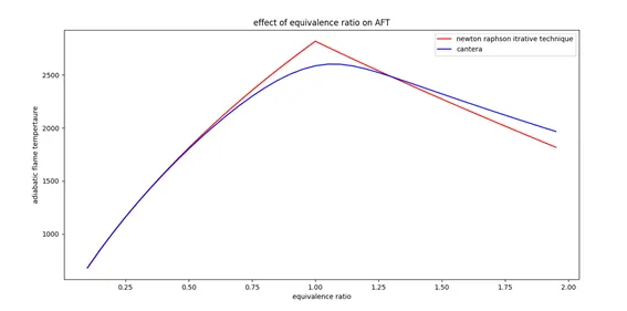
From graph we easily conclude that at equivalence ration equal to 1 stoichiometric condition The AFT is highest. After Stoichiometric AFT is decreased. This is because of in this condition all fuel is burned and then producing more energy
Result got from cantera shows lower AFT than the code using newton Rapson method. The Reason for this cantera considered all the product of combustion which would occure in the actual case.so more energy used to produce products.
Hence AFT is obtained through cantera which is actual solution
Case 2
Coding approach-
The combustion is considered at constant pressure chamber.
For constant constant enthalpy process equation obtaines is
hproduct-hreactant-heatloss=0
heat loss=heat loss factor*LHV
vary heat loss factor varies between 0 to 1
"""
Adaibatic temperature
CH4 + 2(O2+3.76N2) = CO2 +2H2O + 7.52N2
"""
import matplotlib.pyplot as plt
import math
import numpy as np
def h(T,co_effs):
R=8.314 #J/mol.k
a1=co_effs[0]
a2=co_effs[1]
a3=co_effs[2]
a4=co_effs[3]
a5=co_effs[4]
a6=co_effs[5]
return (a1 + a2*T/2 + a3*pow(T,2)/3 + a4*pow(T,3)/4 + a5*pow(T,4)/5 + a6/T)*R*T
CH4_coeffs_l=[5.14987613E+00,-1.36709788E-02,4.91800599E-05 ,-4.84743026E-08 ,1.66693956E-11,-1.02466476E+04,-4.64130376E+00]
O2_coeffs_l=[3.78245636E+00,-2.99673416E-03, 9.84730201E-06 , -9.68129509E-09,3.24372837E-12,-1.06394356E+03 ,3.65767573E+00]
N2_coeffs_l=[0.03298677E+02, 0.14082404E-02,-0.03963222E-04, 0.05641515E-07,-0.02444854E-10,-0.10208999E+04, 0.03950372E+02]
CO2_coeffs_h=[3.85746029E+00, 4.41437026E-03,-2.21481404E-06, 5.23490188E-10,-4.72084164E-14,-4.87591660E+04,2.27163806E+00]
H2O_coeffs_h=[3.03399249E+00, 2.17691804E-03,-1.64072518E-07,-9.70419870E-11, 1.68200992E-14, -3.00042971E+04, 4.96677010E+00]
N2_coeffs_h=[0.02926640E+02 ,0.14879768E-02,-0.05684760E-05 ,0.10097038E-09,-0.06753351E-13,-0.09227977E+04, 0.05980528E+02]
def f(T):
h_CO2_p=h(T,CO2_coeffs_h)
h_H2O_p=h(T,H2O_coeffs_h)
h_N2_p=h(T,N2_coeffs_h)
hproduct=h_CO2_p +2*h_H2O_p+7.52*h_N2_p
Tstd=298.15
LHV=800000
h_CH4_r=h(Tstd,CH4_coeffs_l)
h_N2_r=h(Tstd,N2_coeffs_l)
h_O2_r=h(Tstd,O2_coeffs_l)
hreactant=h_CH4_r + 2*h_O2_r +7.52*h_N2_r
return hproduct - hreactant +L*LHV
def fprime(T):
return (f(T +1e-6)-f(T))/1e-6
T_guess=1500
tol = 1e-3
ct=0
alpha=0.2
for L in np.arange(0,1,0.1):
while (abs(f(T_guess))>tol):
T_guess=T_guess -alpha*(f(T_guess)/fprime(T_guess))
ct=ct+1
plt.plot(L,T_guess,'o',color='blue')
plt.grid ()
plt.xlabel('heat loss factor')
plt.ylabel('adiabatic flame tempertaure')
plt.title('effect of heat loss factor on AFT')
plt.show()
Results
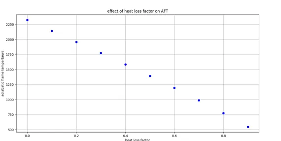
From the graph AFT decreases as heat loss factor increases and this is because of less energy is contained in the chamber thereby reducing the temperture
Case 3
Coding approach
The same approach is consider was formed and tested for -ane,ene,yne variant of 2 carbon atom chain. The hydrocarbon are ethane, ethane, ethyne
"""
Adaibatic temperature
CxHy + (x+y/4)(O2+3.76N2) = xCO2 +y/2H2O + (x+y/4)3.76N2
"""
import matplotlib.pyplot as plt
import math
import numpy as np
def h(T,co_effs):
R=8.314 #J/mol.k
a1=co_effs[0]
a2=co_effs[1]
a3=co_effs[2]
a4=co_effs[3]
a5=co_effs[4]
a6=co_effs[5]
return (a1 + a2*T/2 + a3*pow(T,2)/3 + a4*pow(T,3)/4 + a5*pow(T,4)/5 + a6/T)*R*T
CH4_coeffs_l=[5.14987613E+00,-1.36709788E-02,4.91800599E-05 ,-4.84743026E-08 ,1.66693956E-11,-1.02466476E+04,-4.64130376E+00]
C2H6_coeffs_l=[4.29142492E+00,-5.50154270E-03, 5.99438288E-05,-7.08466285E-08, 2.68685771E-11,-1.15222055E+04, 2.66682316E+00]
C2H4_coeffs_l=[3.95920148E+00,-7.57052247E-03, 5.70990292E-05, -6.91588753E-08, 2.69884373E-11, 5.08977593E+03, 4.09733096E+00 ]
C2H2_coeffs_l=[8.08681094E-01, 2.33615629E-02,-3.55171815E-05,2.80152437E-08,-8.50072974E-12, 2.64289807E+04, 1.39397051E+01]
C3H8_coeffs_l=[ 0.93355381E+00, 0.26424579E-01, 0.61059727E-05, -0.21977499E-07, 0.95149253E-11,-0.13958520E+05, 0.19201691E+02]
O2_coeffs_l=[3.78245636E+00,-2.99673416E-03, 9.84730201E-06 , -9.68129509E-09,3.24372837E-12,-1.06394356E+03 ,3.65767573E+00]
N2_coeffs_l=[0.03298677E+02, 0.14082404E-02,-0.03963222E-04, 0.05641515E-07,-0.02444854E-10,-0.10208999E+04, 0.03950372E+02]
CO2_coeffs_h=[3.85746029E+00, 4.41437026E-03,-2.21481404E-06, 5.23490188E-10,-4.72084164E-14,-4.87591660E+04,2.27163806E+00]
H2O_coeffs_h=[3.03399249E+00, 2.17691804E-03,-1.64072518E-07,-9.70419870E-11, 1.68200992E-14, -3.00042971E+04, 4.96677010E+00]
N2_coeffs_h=[0.02926640E+02 ,0.14879768E-02,-0.05684760E-05 ,0.10097038E-09,-0.06753351E-13,-0.09227977E+04, 0.05980528E+02]
def f(T):
h_CO2_p=h(T,CO2_coeffs_h)
h_H2O_p=h(T,H2O_coeffs_h)
h_N2_p=h(T,N2_coeffs_h)
hproduct=x*h_CO2_p +(y/2)*h_H2O_p+(x+y/4)*3.76*h_N2_p
Tstd=298.15
h_C2H6_r=h(Tstd,C2H6_coeffs_l)
h_N2_r=h(Tstd,N2_coeffs_l)
h_O2_r=h(Tstd,O2_coeffs_l)
h_C2H4_r=h(Tstd,C2H4_coeffs_l)
h_C2H2_r=h(Tstd,C2H2_coeffs_l)
if y==y_ane:
LHV=1428600
hreactant=h_C2H6_r + (x+y/4)*h_O2_r +(x+y/4)*3.76*h_N2_r
if y==y_ene:
LHV=1227070
hreactant=h_C2H4_r + (x+y/4)*h_O2_r +(x+y/4)*3.76*h_N2_r
if y==y_yne:
LHV=1157784
hreactant=h_C2H2_r + (x+y/4)*h_O2_r +(x+y/4)*3.76*h_N2_r
return hproduct - hreactant +0.35*LHV
def fprime(T):
return (f(T +1e-6)-f(T))/1e-6
T_guess=1500
tol = 1e-3
ct=0
alpha=0.5
x=2
y_ane=2*x+2
y_ene=2*x
y_yne=2*x-2
y1=[y_ane,y_ene,y_yne]
fuel=['ethane','ethene','ethyne']
T_adibatic=[]
for y in y1:
while (abs(f(T_guess))>tol):
T_guess=T_guess -alpha*(f(T_guess)/fprime(T_guess))
ct=ct+1
T_adibatic.append(T_guess)
print (ct)
print (T_guess)
plt.bar (fuel,T_adibatic)
plt.xlabel('hydrocarbon')
plt.ylabel('adiabatic flame tempertaure')
plt.title('effect of types hydrocarbon on AFT')
plt.show()
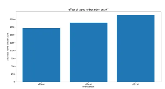
The AFT for ethane=1714 k, ethane=1890k, ethyne=2133k was obtained
From the bar graph AFT is higher in case ethyne and lowest in case ethane. Because ethyne has triple bond higher energy is required to produce product
Case 4
The carbon atoms are varied from 1 to 3 for the alkane group and the AFT is compared between them. The hydrocarbon is Methane, ethane and propane. Heat loss Factor taken is 0
"""
Adaibatic temperature
CxHy + (x+y/4)(O2+3.76N2) = xCO2 +y/2H2O + (x+y/4)3.76N2
"""
import matplotlib.pyplot as plt
import math
import numpy as np
def h(T,co_effs):
R=8.314 #J/mol.k
a1=co_effs[0]
a2=co_effs[1]
a3=co_effs[2]
a4=co_effs[3]
a5=co_effs[4]
a6=co_effs[5]
return (a1 + a2*T/2 + a3*pow(T,2)/3 + a4*pow(T,3)/4 + a5*pow(T,4)/5 + a6/T)*R*T
CH4_coeffs_l=[5.14987613E+00,-1.36709788E-02,4.91800599E-05 ,-4.84743026E-08 ,1.66693956E-11,-1.02466476E+04,-4.64130376E+00]
C2H6_coeffs_l=[4.29142492E+00,-5.50154270E-03, 5.99438288E-05,-7.08466285E-08, 2.68685771E-11,-1.15222055E+04, 2.66682316E+00]
C3H8_coeffs_l=[ 0.93355381E+00, 0.26424579E-01, 0.61059727E-05, -0.21977499E-07, 0.95149253E-11,-0.13958520E+05, 0.19201691E+02]
O2_coeffs_l=[3.78245636E+00,-2.99673416E-03, 9.84730201E-06 , -9.68129509E-09,3.24372837E-12,-1.06394356E+03 ,3.65767573E+00]
N2_coeffs_l=[0.03298677E+02, 0.14082404E-02,-0.03963222E-04, 0.05641515E-07,-0.02444854E-10,-0.10208999E+04, 0.03950372E+02]
CO2_coeffs_h=[3.85746029E+00, 4.41437026E-03,-2.21481404E-06, 5.23490188E-10,-4.72084164E-14,-4.87591660E+04,2.27163806E+00]
H2O_coeffs_h=[3.03399249E+00, 2.17691804E-03,-1.64072518E-07,-9.70419870E-11, 1.68200992E-14, -3.00042971E+04, 4.96677010E+00]
N2_coeffs_h=[0.02926640E+02 ,0.14879768E-02,-0.05684760E-05 ,0.10097038E-09,-0.06753351E-13,-0.09227977E+04, 0.05980528E+02]
def f(T):
h_CO2_p=h(T,CO2_coeffs_h)
h_H2O_p=h(T,H2O_coeffs_h)
h_N2_p=h(T,N2_coeffs_h)
hproduct=x*h_CO2_p +(y/2)*h_H2O_p+(x+y/4)*3.76*h_N2_p
Tstd=298.15
h_CH4_r=h(Tstd,CH4_coeffs_l)
h_N2_r=h(Tstd,N2_coeffs_l)
h_O2_r=h(Tstd,O2_coeffs_l)
h_C2H6_r=h(Tstd,C2H6_coeffs_l)
h_C3H8_r=h(Tstd,C3H8_coeffs_l)
if x==1:
hreactant=h_CH4_r + (x+y/4)*h_O2_r +(x+y/4)*3.76*h_N2_r
if x==2:
hreactant=h_C2H6_r + (x+y/4)*h_O2_r +(x+y/4)*3.76*h_N2_r
if x==3:
hreactant=h_C3H8_r + (x+y/4)*h_O2_r +(x+y/4)*3.76*h_N2_r
return hproduct - hreactant
def fprime(T):
return (f(T +1e-6)-f(T))/1e-6
T_guess=1500
tol = 1e-3
ct=0
alpha=0.2
fuel=['methane','ethane','propane']
T_adibatic=[]
for x in range (1,4):
y=2*x+2
while (abs(f(T_guess))>tol):
T_guess=T_guess -alpha*(f(T_guess)/fprime(T_guess))
ct=ct+1
T_adibatic.append(T_guess)
print (ct)
print (T_guess)
plt.bar (fuel,T_adibatic)
plt.xlabel('hydrocarbon')
plt.ylabel('adiabatic flame tempertaure')
plt.title('effect of types hydrocarbon on AFT')
plt.show()
Results-
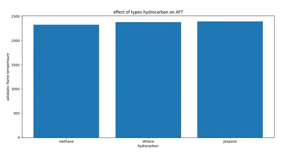
AFT for Methane=2325.6k, Ethane=2379.8k, Propane=2392K
From the graph we see that propane has highest AFT while methane has lowest AFT .so it is concluding that AFT is increase with increasing no. of carbon atoms for alkane group of hydro carbon