Week 3 - Adiabatic Flame Temperature calculation
AIM:
- Adiabatic flame temperature at different equivalence ratio (Const. volume)
- Adiabatic flame temperature at different heat loss fraction (Const. pressure)
- Adiabatic flame temperature for hydrocarbons with 2 carbon atoms
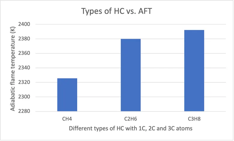
- Adiabatic flame temperature for hydrocarbons upto 3 carbon atom chains
INTRODUCTION and THEORY:
Adiabatic flame temperature:
The adiabatic flame temperature is the maximum temperature attained by the chemical species involved in the combustion reaction under no heat loss to the surroundings. The flame temperature can be obtained at constant volume or constant pressure. But the constant volume process of flame temperature is higher than the constant pressure process.
At constant volume:
deltaU = 0
Hreactants - Hproducts – R(Nreactants.Tstd – Nproducts.Taft)= 0
At constant pressure:
deltaH = 0
Hreactants - Hproducts = 0
The highest adiabatic flame temperature is achieved at the equivalence ratio of 1. If the initial fuel or air changes from stoichiometric conditions then the equivalence ratio of the reaction changes and lowers the adiabatic flame temperature. It shows that the flame temperature highly depends on the equivalence ratio of the chemical reaction. In addition to this, it also depends on the heat loss, number of C and H atoms present in the fuel.
Newton-Raphson method:
The Newton raphson technique is used to solve the nonlinear equation by linear approximation. This method is helpful to find out the roots of the nonlinear equation. By continuous iteration this method solves the equation with good approximation.
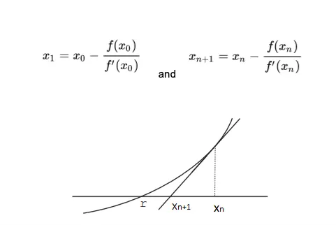
To calculate the adiabatic flame temperature the function at constant volume or constant pressure should be equal to 0. This can be obtained by the Newton raphson method.
Equivalence ratio:
The equivalence ratio is the ratio of fuel/air ratio to the stoichiometric fuel/air ratio.
Equivalence ratio = { (Air/Fuel)sto / (Air/Fuel) }
If equivalence ratio = 1; Stoichiometric mixture
If equivalence ratio > 1; Rich mixture
If equilvaence ratio < 1; Lean mixture
Practical applications:
In coal combustion systems, calculating flame temperature is essential. This is due to the fact that more oxygen is added to the combustion chambers for complete combustion of the coal. This deviates the overall heat generation and it's highly risky in large-scale applications.
CODING APPROACH:
Part 1: Coefficient parameters
For calculating the enthalpy of our reaction we need to define polynomial coefficients of species involved in products and reactants. Using the GRI thermo file the coefficients are extracted and defined as an array. For reactants first 7 coefficients are used and for products last 7 coefficients are used.
Part 2: Enthalpy calculation
It is important to calculate the enthalpy of each species in products and reactants of the reaction. For that we define the function with input values temperature (T) and polynomial coefficients which have been extracted before as co_effs. The return value of this function calculates the enthalpy of individual species present in products and reactants.
Part 3: Finding value for f(T)
Finding the roots of nonlinear equations is an important objective of our project. Before that, we need to find the value for f(T) which is essential to find adiabatic flame temperature. For that, we define the function with T and call the function h(T, co_effs) defined above using polynomial coefficient values of individual species and calculate the overall enthalpy of the reaction. The reactants are involved in the low temperature region as a result the initialization temperature Tstd is set at 298.15K.
Part 4: Newton Raphson method
For iterative and root finding problems we need Newton Raphson technique. Using this method we are solving the nonlinear equation with linear approximation. In this section we use the Newton raphson formula for finding the adiabatic temperature value using the function f(T), fprime, and alpha. The fprime is the numerical derivative of the function f(T) using the forward differencing technique. Alpha is the under relaxation parameter and it should be between 0 to 1. The value is calculated inside the while loop for continuous iterative process and if the iteration goes beyond tolerance value the loop stops. Using the print command the final adiabatic final temperature is calculated.
CODE and RESULTS:
Question 1: AFT at different equivalence ratio (Const. volume)
EQ 0.6 = CH4 + 3.33 (O2 + 3.76 N2) => CO2 + 2H2O + 12.53 N2 + 1.33 O2
EQ 0.8 = CH4 + 2.5 (O2 + 3.76 N2) => CO2 + 2H2O + 9.4 N2 + 0.5 O2
EQ 1 = CH4 + 2(O2 + 3.76 N2) => CO2 + 2H2O + 7.52 N2
EQ 1.2 = CH4 + 1.67(O2 + 3.76 N2) => 0.33 CO2 + 2H2O + 6.26 N2 + 0.67 CO
Code for EQ 0.8
Python:
import matplotlib.pyplot as plt
import numpy as np
def h(T, co_effs):
R = 8.314 #J/mok-K
a1 = co_effs[0]
a2 = co_effs[1]
a3 = co_effs[2]
a4 = co_effs[3]
a5 = co_effs[4]
a6 = co_effs[5]
return(a1 + a2*T/2 + a3*pow(T,2)/3 + a4*pow(T,3)/4 + a5*pow(T,4)/5 + a6/T)*R*T
ch4_coeffs_l = [5.14987613E+00, -1.36709788E-02, 4.91800599E-05, -4.84743026E-08, 1.66693956E-11, -1.02466476E+04]
o2_coeffs_l = [3.78245636E+00, -2.99673416E-03, 9.84730201E-06, -9.68129509E-09, 3.24372837E-12, -1.06394356E+03]
n2_coeffs_l = [0.03298677E+02, 0.14082404E-02, -0.03963222E-04, 0.05641515E-07, -0.02444854E-10, -0.10208999E+04]
co2_coeffs_h = [3.85746029E+00, 4.41437026E-03, -2.21481404E-06, 5.23490188E-10, -4.72084164E-14, -4.87591660E+04]
h2o_coeffs_h = [3.03399249E+00, 2.17691804E-03, -1.64072518E-07, -9.70419870E-11, 1.68200992E-14, -3.00042971E+04]
n2_coeffs_h = [0.02926640E+02, 0.14879768E-02, -0.05684760E-05, 0.10097038E-09, -0.06753351E-13, -0.09227977E+04]
o2_coeffs_h = [3.28253784E+00, 1.48308754E-03, -7.57966669E-07, 2.09470555E-10, -2.16717794E-14, -1.08845772E+03]
def f(T):
R = 8.314 #J/mok-K
h_co2_prod = h(T, co2_coeffs_h)
h_h2o_prod = h(T, h2o_coeffs_h)
h_n2_prod = h(T, n2_coeffs_h)
h_o2_prod = h(T,o2_coeffs_h)
H_products = h_co2_prod + 2*(h_h2o_prod) + 9.4*(h_n2_prod) + 0.5*(h_o2_prod)
N_products = (1 + 2 + 9.4 + 0.5)
Tstd = 298.15
h_ch4_reac = h(Tstd, ch4_coeffs_l)
h_o2_reac = h(Tstd, o2_coeffs_l)
h_n2_reac = h(Tstd, n2_coeffs_l)
H_reactants = h_ch4_reac + 2.5*(h_o2_reac) + 9.4*(h_n2_reac)
N_reactants = (1 + 2.5 + 9.4)
print(H_reactants - H_products - R*(N_reactants*Tstd - N_products*T))
return H_reactants - H_products - R*(N_reactants*Tstd - N_products*T)
def fprime(T):
return(f(T+1e-6) - f(T))/1e-6
T_guess = 1500
tol = 1e-3
ct = 0
alpha = 0.2
while(abs(f(T_guess)) > tol):
T_guess = T_guess - alpha*((f(T_guess)/fprime(T_guess)))
plt.plot(ct,T_guess, '*r')
ct = ct+1
print(ct)
print(T_guess)
plt.show()
Cantera:
import cantera as ct
gas = ct.Solution('grimech30.cti')
gas.TPX = 298.15, 101325, 'CH4:1, O2:2.5, N2:9.4'
gas.equilibrate('UV','auto')
print(gas.T)
Results:
|
Equivalence ratio |
AFT Python (K) |
AFT Cantera (K) |
|
0.6 |
2041.03 |
2019.67 |
|
0.8 |
2452.46 |
2377.51 |
|
1 |
2817.83 |
2585.88 |
|
1.2 |
2591.51 |
2558 |
Plotting python and Cantera:
import matplotlib.pyplot as plt
Equ = [0.6, 0.8, 1.0, 1.2]
py = [2041.028783, 2452.459889, 2817.831019, 2591.513873]
ca = [2019.66507, 2377.513793, 2585.878267, 2557.996425]
plt.figure()
plt.plot(Equ, py, '-r', label='Python')
plt.plot(Equ, ca, '-b', label='Cantera')
plt.xlabel('Equivalence ratio')
plt.ylabel('Adiabatic flame temperature in K')
plt.legend(loc=0)
plt.savefig('AFTcalc.png')
plt.show()
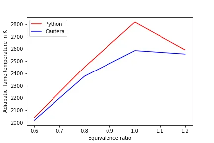
- It is evident from the graph that the temperature of Python is higher than the Cantera flame temperature at different equivalence ratios.
- The peak temperature at the equivalence ratio of 1 for both Python and Cantera.
- Cantera uses Gibbs minimization method for calculating adiabatic flame temperature. Moreover, Cantera assumes products of large number of species whereas Python calculates temperature for 3 product species only. Higher number of products lower the flame temperature.
Question 2: AFT at different heat loss fraction (Const. pressure)
Equation: CH4 + 2(O2 + 3.76 N2) => CO2 + 2H2O + 7.52 N2
Heat loss fraction at 1:
import matplotlib.pyplot as plt
import numpy as np
def h(T, co_effs):
R = 8.314 #J/mok-K
a1 = co_effs[0]
a2 = co_effs[1]
a3 = co_effs[2]
a4 = co_effs[3]
a5 = co_effs[4]
a6 = co_effs[5]
return(a1 + a2*T/2 + a3*pow(T,2)/3 + a4*pow(T,3)/4 + a5*pow(T,4)/5 + a6/T)*R*T
ch4_coeffs_l = [5.14987613E+00, -1.36709788E-02, 4.91800599E-05, -4.84743026E-08, 1.66693956E-11, -1.02466476E+04]
o2_coeffs_l = [3.78245636E+00, -2.99673416E-03, 9.84730201E-06, -9.68129509E-09, 3.24372837E-12, -1.06394356E+03]
n2_coeffs_l = [0.03298677E+02, 0.14082404E-02, -0.03963222E-04, 0.05641515E-07, -0.02444854E-10, -0.10208999E+04]
co2_coeffs_h = [3.85746029E+00, 4.41437026E-03, -2.21481404E-06, 5.23490188E-10, -4.72084164E-14, -4.87591660E+04]
h2o_coeffs_h = [3.03399249E+00, 2.17691804E-03, -1.64072518E-07, -9.70419870E-11, 1.68200992E-14, -3.00042971E+04]
n2_coeffs_h = [0.02926640E+02, 0.14879768E-02, -0.05684760E-05, 0.10097038E-09, -0.06753351E-13, -0.09227977E+04]
def f(T):
R = 8.314 #J/mok-K
h_co2_prod = h(T, co2_coeffs_h)
h_h2o_prod = h(T, h2o_coeffs_h)
h_n2_prod = h(T, n2_coeffs_h)
H_products = h_co2_prod + 2*(h_h2o_prod) + 7.52*(h_n2_prod)
Tstd = 298.15
h_ch4_reac = h(Tstd, ch4_coeffs_l)
h_o2_reac = h(Tstd, o2_coeffs_l)
h_n2_reac = h(Tstd, n2_coeffs_l)
H_reactants = h_ch4_reac + 2*(h_o2_reac) + 7.52*(h_n2_reac)
return ((H_products - H_reactants) + (1.0 * 802300))
def fprime(T):
return(f(T+1e-6) - f(T))/1e-6
T_guess = 1500
tol = 1e-3
ct = 0
alpha = 0.2
while(abs(f(T_guess)) > tol):
T_guess = T_guess - alpha*((f(T_guess)/fprime(T_guess)))
plt.plot(ct,T_guess, '*r')
ct = ct+1
print(ct)
print(T_guess)
plt.show()
Results:
|
Heat loss factor |
AFT (K) |
|
0 |
2325.6 |
|
0.1 |
2143.61 |
|
0.2 |
1959.59 |
|
0.3 |
1773.02 |
|
0.4 |
1583.26 |
|
0.5 |
1389.44 |
|
0.6 |
1190.39 |
|
0.7 |
984.508 |
|
0.8 |
769.455 |
|
0.9 |
541.652 |
|
1 |
295.101 |
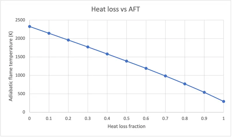
It is obvious that an increase in heat loss fraction lowers the AFT. Would like to mention again, AFT is the maximum temperature with no heat loss in the system.
Question 3: AFT of various hydrocarbons with 2 Carbon atoms
Alkane (Ethane): C2H6 + 3.5(O2 + 3.76N2) => 2CO2 + 3H2O + 3.76(3.5)N2
Alkene (Ethene or Ethylene): C2H4 + 3(O2 + 3.76N2) => 2CO2 + 2H2O + 3.76*3*N2
Alkyne (Acetylene): C2H2 + 2.5(O2 + 3.76N2) => 2CO2 + H2O + 3.76*2.5*N2
Code for alkane:
import matplotlib.pyplot as plt
import numpy as np
# C2H6 + 3.5(O2 + 3.76N2) => 2CO2 + 3H2O + 3.76(3.5)N2
def h(T, co_effs):
R = 8.314 #J/mok-K
a1 = co_effs[0]
a2 = co_effs[1]
a3 = co_effs[2]
a4 = co_effs[3]
a5 = co_effs[4]
a6 = co_effs[5]
return(a1 + a2*T/2 + a3*pow(T,2)/3 + a4*pow(T,3)/4 + a5*pow(T,4)/5 + a6/T)*R*T
c2h6_coeffs_l = [4.29142492E+00, -5.50154270E-03, 5.99438288E-05, -7.08466285E-08, 2.68685771E-11, -1.15222055E+04]
o2_coeffs_l = [3.78245636E+00, -2.99673416E-03, 9.84730201E-06, -9.68129509E-09, 3.24372837E-12, -1.06394356E+03]
n2_coeffs_l = [0.03298677E+02, 0.14082404E-02, -0.03963222E-04, 0.05641515E-07, -0.02444854E-10, -0.10208999E+04]
co2_coeffs_h = [3.85746029E+00, 4.41437026E-03, -2.21481404E-06, 5.23490188E-10, -4.72084164E-14, -4.87591660E+04]
h2o_coeffs_h = [3.03399249E+00, 2.17691804E-03, -1.64072518E-07, -9.70419870E-11, 1.68200992E-14, -3.00042971E+04]
n2_coeffs_h = [0.02926640E+02, 0.14879768E-02, -0.05684760E-05, 0.10097038E-09, -0.06753351E-13, -0.09227977E+04]
def f(T):
R = 8.314 #J/mok-K
h_co2_prod = h(T, co2_coeffs_h)
h_h2o_prod = h(T, h2o_coeffs_h)
h_n2_prod = h(T, n2_coeffs_h)
H_products = 2*h_co2_prod + 3*(h_h2o_prod) + 3.76*3.5*(h_n2_prod)
N_products = (2 + 3 + (3.76*3.5))
Tstd = 298.15
h_c2h6_reac = h(Tstd, c2h6_coeffs_l)
h_o2_reac = h(Tstd, o2_coeffs_l)
h_n2_reac = h(Tstd, n2_coeffs_l)
H_reactants = 1*h_c2h6_reac + 3.5*(h_o2_reac) + 3.76*3.5*(h_n2_reac)
N_reactants = (1 + 3.5 + 3.76)
return H_products - H_reactants #- R*(N_reactants*Tstd - N_products*T)
def fprime(T):
return(f(T+1e-6) - f(T))/1e-6
T_guess = 1500
tol = 1e-3
ct = 0
alpha = 0.2
while(abs(f(T_guess)) > tol):
T_guess = T_guess - alpha*((f(T_guess)/fprime(T_guess)))
plt.plot(ct,T_guess, '*r')
ct = ct+1
print(ct)
print(T_guess)
plt.show()
Results:
|
Types of Hydrocarbons |
AFT (K) |
|
|
Alkane |
Ethane |
2379.85 |
|
Alkene |
Ethylene |
2564.53 |
|
Alkyne |
Acetylene |
2909.35 |
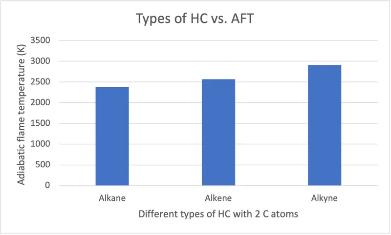
Higher the bond, higher energy is released from it.
Question 4: AFT vs number of C atoms
1 C : CH4 + 2(O2 + 3.76N2) => CO2 + 2H2O + 3.72*2*N2
2 C: C2H6 + 3.5(O2 + 3.76N2) => 2CO2 + 3H2O + 3.76(3.5)N2
3 C: C3H8 + 5(O2 + 3.76N2) => 3CO2 + 4H2O + 3.76(5)N2
Code for 1 C:
import matplotlib.pyplot as plt
import numpy as np
# CH4 + 2(O2 + 3.76N2) => CO2 + 2H2O + 3.72*2*N2
def h(T, co_effs):
R = 8.314 #J/mok-K
a1 = co_effs[0]
a2 = co_effs[1]
a3 = co_effs[2]
a4 = co_effs[3]
a5 = co_effs[4]
a6 = co_effs[5]
return(a1 + a2*T/2 + a3*pow(T,2)/3 + a4*pow(T,3)/4 + a5*pow(T,4)/5 + a6/T)*R*T
ch4_coeffs_l = [5.14987613E+00, -1.36709788E-02, 4.91800599E-05, -4.84743026E-08, 1.66693956E-11, -1.02466476E+04]
o2_coeffs_l = [3.78245636E+00, -2.99673416E-03, 9.84730201E-06, -9.68129509E-09, 3.24372837E-12, -1.06394356E+03]
n2_coeffs_l = [0.03298677E+02, 0.14082404E-02, -0.03963222E-04, 0.05641515E-07, -0.02444854E-10, -0.10208999E+04]
co2_coeffs_h = [3.85746029E+00, 4.41437026E-03, -2.21481404E-06, 5.23490188E-10, -4.72084164E-14, -4.87591660E+04]
h2o_coeffs_h = [3.03399249E+00, 2.17691804E-03, -1.64072518E-07, -9.70419870E-11, 1.68200992E-14, -3.00042971E+04]
n2_coeffs_h = [0.02926640E+02, 0.14879768E-02, -0.05684760E-05, 0.10097038E-09, -0.06753351E-13, -0.09227977E+04]
def f(T):
R = 8.314 #J/mok-K
h_co2_prod = h(T, co2_coeffs_h)
h_h2o_prod = h(T, h2o_coeffs_h)
h_n2_prod = h(T, n2_coeffs_h)
H_products = h_co2_prod + 2*(h_h2o_prod) + 7.52*(h_n2_prod)
N_products = (1 + 2 + 7.52)
Tstd = 298.15
h_ch4_reac = h(Tstd, ch4_coeffs_l)
h_o2_reac = h(Tstd, o2_coeffs_l)
h_n2_reac = h(Tstd, n2_coeffs_l)
H_reactants = h_ch4_reac + 2*(h_o2_reac) + 7.52*(h_n2_reac)
N_reactants = (1 + 2 + 7.52)
return H_products - H_reactants
def fprime(T):
return(f(T+1e-6) - f(T))/1e-6
T_guess = 1500
tol = 1e-3
ct = 0
alpha = 0.2
while(abs(f(T_guess)) > tol):
T_guess = T_guess - alpha*((f(T_guess)/fprime(T_guess)))
plt.plot(ct,T_guess, '*r')
ct = ct+1
print(ct)
print(T_guess)
plt.show()
Results:
|
Types of Hydrocarbons |
AFT (K) |
|
|
C = 1 |
CH4 |
2325.6 |
|
C = 2 |
C2H6 |
2379.85 |
|
C = 3 |
C3H8 |
2392.1 |
Conclusion:
It is concluded that for more accurate and precise adiabatic flame temperatures Cantera is used. Moreover, it is evident that flame temperature changes with varying the inlet fuel and air, heat loss ratio and number of carbon and hydrogen atoms in the fuel.