Week 3 - Adiabatic Flame Temperature calculation
Aim: - To calculate Adiabatic Flame Temperature (AFT) for combustion of different hydrocarbons using python.
Objective: -
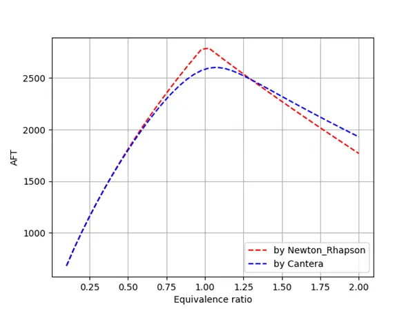
- To plot the variation of AFT to Equivalence ratio for combustion of Methane using Newton-Raphson iterative method and Cantera and compare the result in constant Volume chamber.
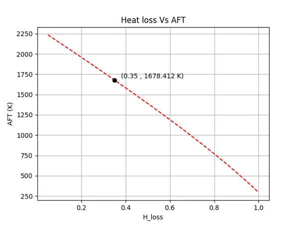
- To plot the variation of AFT to heat loss for combustion of methane in constant pressure chamber using both the methods and compare the results. find AFT for Heat loss coefficient 0.35.
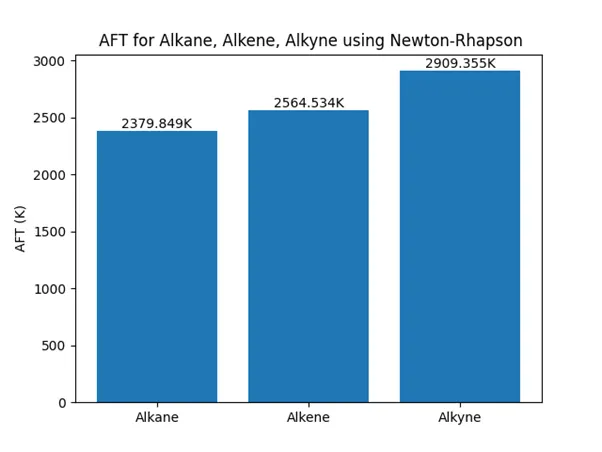
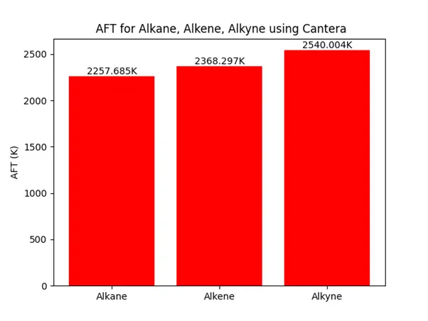
- To find AFT variation with respect to Alkane, Alkene, Alkyne.
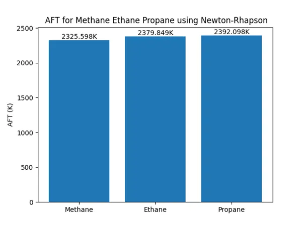
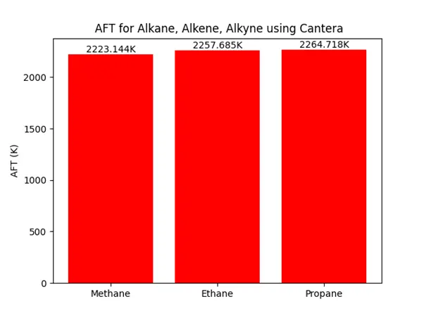
- To find AFT variation with respect to a number of Carbon atom chains up to 3 carbon atoms.
Theory: -
Adiabatic Flame temperature –
In a given combustion process, that takes place adiabatically and with no work or changes in kinetic or potential energy involved, the temperature of the products is referred to as AFT.
It is of type depending on how the process is completed –
- Constant volume AFT - the temperature that results from a complete combustion process that occurs without any work, heat transfer or changes in kinetic or potential energy.
the final equation to be minimised is -
`H_r-H_p-R_u(N_rT_i-N_pT_(ad))=0`
were
Hr = Enthalpy of reactant, Hp = Enthalpy of Product, Ru = 8.314 J/mol-K
Nr = moles of reactant Np= moles of product Ti= 298.15 K
- Constant pressure AFT – the temperature that results from a complete combustion process where all the heat added goes into changing the volume (expansion) of the gas. The final equation to be minimised is –
`ΔH=0`
Equivalence Ratio –
The equivalence ratio is defined as the ratio of the actual fuel/air ratio to the stoichiometric fuel/air ratio.
`ϕ=((Fuel)/(Air))_(Actual )/ ((Fuel)/(Air))_(Stochicometric)`
were,
φ = 1 Stoichiometric mixture
φ < 1 Fuel lean mixture (excess air)
φ > 1 Fuel rich mixture (excess fuel)
Steps –
- Coefficients of elements of combustion are taken from therm.dat from GRI- mech file.
- Enthalpy are calculated using NASA Enthalpy polynomial and using above coefficients.
- A function is F is defined to calculate Enthalpy of product minus Enthalpy of reactants and No of moles for both if required.
- A function fprime is defined which is a forward Differencing scheme.
- A for loop is used to use Newton-Raphson iterative method.
- the finding is plotted.
- To use Cantera an object gas is created.
- Equivalence ration is set for gas along with temperature and pressure.
- Equilibrate function from Cantera is used to find the AFT and appropriately plotted.
case 1 - Equivalence Ratio Vs AFT
Code
"""
 Plotting AFT vs Equivalence Ratio (eq) for methane combustion


  General form stoichiometric equations: CxHy + (x+y/4)(O2+3.76N2) -> xCO2 + (y/2)H2O + (x+y/4)N2

  Lean mixture:  CH4 + (2/eq)(O2+3.76N2) -> CO2 + 2H2O + ((2/eq)-2)O2 + (7.52/eq)N2
  stoichiometric mixture:  CH4 + 2(O2+3.76N2) -->  CO2 + 2H2O + 7.52N2
  Rich Mixture:  CH4 + (2/eq)(O2+3.76N2) -> ((4/eq)-3)CO2 + 2H2O + (4-(4/eq))CO + (7.52/eq)N2

 """
import matplotlib.pyplot as plt
import cantera as ct
import numpy as np
import math


 # Coefficients from nasa therm data, l = lower temp, h = higher temp
coeff_ch4_l = [5.14987613E+00,-1.36709788E-02,4.91800599E-05,-4.84743026E-08,1.66693956E-11,-1.02466476E+04,-4.64130376E+00]
coeff_ch4_h = [7.48514950E-02,1.33909467E-02,-5.73285809E-06,1.22292535E-09,-1.01815230E-13,-9.46834459E+03,1.84373180E+01]
coeff_o2_l = [3.78245636E+00,-2.99673416E-03,9.84730201E-06,-9.68129509E-09,3.24372837E-12,-1.06394356E+03,3.65767573E+00]
coeff_o2_h = [3.28253784E+00,1.48308754E-03,-7.57966669E-07,2.09470555E-10,-2.16717794E-14,-1.08845772E+03,5.45323129E+00]
coeff_n2_l = [0.03298677E+02,0.14082404E-02,-0.03963222E-04,0.05641515E-07,-0.02444854E-10,-0.10208999E+04,0.03950372E+02]
coeff_n2_h = [0.02926640E+02,0.14879768E-02,-0.05684760E-05,0.10097038E-09,-0.06753351E-13,-0.09227977E+04,0.05980528E+02]
coeff_co2_l = [2.35677352E+00,8.98459677E-03,-7.12356269E-06,2.45919022E-09,-1.43699548E-13,-4.83719697E+04,9.90105222E+00]
coeff_co2_h = [3.85746029E+00,4.41437026E-03,-2.21481404E-06,5.23490188E-10,-4.72084164E-14,-4.87591660E+04,2.27163806E+00]
coeff_h2o_l = [4.19864056E+00,-2.03643410E-03,6.52040211E-06,-5.48797062E-09,1.77197817E-12,-3.02937267E+04,-8.49032208E-01]
coeff_h2o_h = [3.03399249E+00,2.17691804E-03,-1.64072518E-07,-9.70419870E-11,1.68200992E-14,-3.00042971E+04,4.96677010E+00]
coeff_co_h = [2.71518561E+00,2.06252743E-03,-9.98825771E-07,2.30053008E-10,-2.03647716E-14,-1.41518724E+04,7.81868772E+00]

#defining Equivaence ration rnge
eq = np.linspace(0.1,2,40)


def h(T,coeffs):

	R = 8.314 #J/mol-K
	a1 = coeffs[0]
	a2 = coeffs[1]
	a3 = coeffs[2]
	a4 = coeffs[3]
	a5 = coeffs[4]
	a6 = coeffs[5]

	return (a1 + a2*T/2 + a3*pow(T,2)/3 + a4*pow(T,3)/4 + a5*pow(T,4)/5 + a6/T)*R*T

def f(T,eq):

	Tstd = 298.15 # K
	R = 8.314 #J/mol-K

    #  enthalpy of Reactant

	h_ch4_r = h(Tstd,coeff_ch4_l)
	h_o2_r = h(Tstd,coeff_o2_l)
	h_n2_r = h(Tstd,coeff_n2_l)

	# enthalpy of products

	h_co2_p = h(T,coeff_co2_h)
	h_h2o_p = h(T,coeff_h2o_h)
	h_n2_p = h(T,coeff_n2_h)
	h_co_p = h(T,coeff_co_h)
	h_o2_p = h(T,coeff_o2_h)

	#reactant
	h_r = h_ch4_r + (2/eq)*h_o2_r + (7.52/eq)*h_n2_r
	n_r = (1 + (2/eq) + (7.52/eq))*R*Tstd

	if eq <= 1:
		# product
		h_p = h_co2_p + 2*h_h2o_p + ((2/eq)-2)*h_o2_p + (7.52/eq)*h_n2_p
		n_p = ( 1 + 2 + ((2/eq)-2) + (7.52/eq))*R*T

	else:
		# product
		h_p = ((4/eq)-3)*h_co2_p + 2*h_h2o_p + (4-(4/eq))*h_co_p + (7.52/eq)*h_n2_p
		n_p = ( ((4/eq)-3) + 2 + (4-(4/eq)) + (7.52/eq))*R*T

	return (h_p - n_p) - (h_r - n_r)

def fprime(T,eq):
	return ((f(T+1e-6,eq) - f(T,eq))/1e-6)


tol = 1e-3
alpha=0.5
T_py=[]


# using Newton-Rhapson Method

for i in range(0,len(eq)):
	T_guess = 2000
	while(abs(f(T_guess,eq[i])) > tol):
		T_guess = T_guess - alpha*((f(T_guess,eq[i])/fprime(T_guess,eq[i])))
	T_py.append(T_guess)

print(max(T_py))

# Using Cantera

gas = ct.Solution('gri30.xml')
T_ct=[]

for i in range(0,len(eq)):
	gas.set_equivalence_ratio(eq[i], 'CH4', 'O2:1.0, N2:3.76')
	gas.TP = 298.15,101325
	gas.equilibrate('UV','auto')
	T_ct.append(gas.T)

print(max(T_ct))

plt.plot(eq,T_py,'--',color='red',label= 'by Newton_Rhapson')
plt.plot(eq,T_ct,'--',color='blue',label= 'by Cantera')
plt.legend(loc='lower right')
plt.xlabel('Equivalence ratio')
plt.ylabel('AFT')
plt.grid('on')
plt.show()
Result: -
Case 2: Heat loss Vs AFT
Code
"""
 Calculating AFT vs heat loss variation for methane combustion

  CH4 + 2(O2+3.76N2) -->  CO2 + 2H2O + 7.52N2

 """
import matplotlib.pyplot as plt
import numpy as np
import math

 # Coefficients from nasa therm data
coeff_ch4_l = [5.14987613E+00,-1.36709788E-02,4.91800599E-05,-4.84743026E-08,1.66693956E-11,-1.02466476E+04,-4.64130376E+00]
coeff_ch4_h = [7.48514950E-02,1.33909467E-02,-5.73285809E-06,1.22292535E-09,-1.01815230E-13,-9.46834459E+03,1.84373180E+01]
coeff_o2_l = [3.78245636E+00,-2.99673416E-03,9.84730201E-06,-9.68129509E-09,3.24372837E-12,-1.06394356E+03,3.65767573E+00]
coeff_o2_h = [3.28253784E+00,1.48308754E-03,-7.57966669E-07,2.09470555E-10,-2.16717794E-14,-1.08845772E+03,5.45323129E+00]
coeff_n2_l = [0.03298677E+02,0.14082404E-02,-0.03963222E-04,0.05641515E-07,-0.02444854E-10,-0.10208999E+04,0.03950372E+02]
coeff_n2_h = [0.02926640E+02,0.14879768E-02,-0.05684760E-05,0.10097038E-09,-0.06753351E-13,-0.09227977E+04,0.05980528E+02]
coeff_co2_l = [2.35677352E+00,8.98459677E-03,-7.12356269E-06,2.45919022E-09,-1.43699548E-13,-4.83719697E+04,9.90105222E+00]
coeff_co2_h = [3.85746029E+00,4.41437026E-03,-2.21481404E-06,5.23490188E-10,-4.72084164E-14,-4.87591660E+04,2.27163806E+00]
coeff_h2o_l = [4.19864056E+00,-2.03643410E-03,6.52040211E-06,-5.48797062E-09,1.77197817E-12,-3.02937267E+04,-8.49032208E-01]
coeff_h2o_h = [3.03399249E+00,2.17691804E-03,-1.64072518E-07,-9.70419870E-11,1.68200992E-14,-3.00042971E+04,4.96677010E+00]


def h(T,coeffs):

	R = 8.314 #J/mol-K
	a1 = coeffs[0]
	a2 = coeffs[1]
	a3 = coeffs[2]
	a4 = coeffs[3]
	a5 = coeffs[4]
	a6 = coeffs[5]

	return (a1 + a2*T/2 + a3*pow(T,2)/3 + a4*pow(T,3)/4 + a5*pow(T,4)/5 + a6/T)*R*T

# coefficient of heat loss
H_loss = np.linspace(.05,1,20)

def f(T,H_loss):

	#  enthalpy of Reactant

	Tstd = 298.15 # K
	h_ch4_r = h(Tstd,coeff_ch4_l)
	h_o2_r = h(Tstd,coeff_o2_l)
	h_n2_r = h(Tstd,coeff_n2_l)

	h_r = h_ch4_r + 2*h_o2_r + 7.52*h_n2_r

	# enthalpy of products

	h_co2_p = h(T,coeff_co2_h)
	h_h2o_p = h(T,coeff_h2o_h)
	h_n2_p = h(T,coeff_n2_h)

	h_p = h_co2_p + 2*h_h2o_p + 7.52*h_n2_p

	# max possible heat loss for system to reach at STP

	qmax = (h_ch4_r + 2*h_o2_r) - (h(Tstd,coeff_co2_l) + 2*h(Tstd,coeff_h2o_l))

	return h_p - h_r + (H_loss*qmax)

def fprime(T,H_loss):
	return ((f(T+1e-6,H_loss) - f(T,H_loss))/1e-6)

tol = 1e-3
alpha=0.5
T_hl=[]


# using Newton-Rhapson Method

for i in range(0,len(H_loss)):
	T_guess = 2000
	while(abs(f(T_guess,H_loss[i])) > tol):
		T_guess = T_guess - alpha*((f(T_guess,H_loss[i])/fprime(T_guess,H_loss[i])))
	T_hl.append(T_guess)

print(H_loss,T_hl)

plt.plot(H_loss,T_hl,'--',color='red')
plt.plot(H_loss[6],T_hl[6],'o',color='black')
plt.xlabel('H_loss')
plt.ylabel('AFT (K)')
plt.title('Heat loss Vs AFT')
plt.text(0.38,1700,'({0:.2f} , {1:.3f} K)'.format(H_loss[6],T_hl[6]))
plt.grid('on')
plt.show()
Result:-
Case 3: - AFT variation with respect to Alkane, Alkene, Alkyne
code
"""
3. Adiabatic flame temperature variation with respect to Alkane, Alkene, Alkyne

General form stoichiometric equations: CxHy + (x+y/4)(O2+3.76N2) -> xCO2 + (y/2)H2O + ((x+y/4)*3.76)N2
"""
import matplotlib.pyplot as plt
import cantera as ct
import numpy as np
import math

coeff_c2h6_l = [4.29142492E+00,-5.50154270E-03,5.99438288E-05,-7.08466285E-08,2.68685771E-11,-1.15222055E+04,2.66682316E+00]
coeff_c2h4_l = [3.95920148E+00,-7.57052247E-03,5.70990292E-05,-6.91588753E-08,2.69884373E-11,5.08977593E+03,4.09733096E+00 ]
coeff_c2h2_l = [8.08681094E-01,2.33615629E-02,-3.55171815E-05,2.80152437E-08,-8.50072974E-12,2.64289807E+04,1.39397051E+01]

coeff_o2_l = [3.78245636E+00,-2.99673416E-03,9.84730201E-06,-9.68129509E-09,3.24372837E-12,-1.06394356E+03,3.65767573E+00]
coeff_o2_h = [3.28253784E+00,1.48308754E-03,-7.57966669E-07,2.09470555E-10,-2.16717794E-14,-1.08845772E+03,5.45323129E+00]
coeff_n2_l = [0.03298677E+02,0.14082404E-02,-0.03963222E-04,0.05641515E-07,-0.02444854E-10,-0.10208999E+04,0.03950372E+02]
coeff_n2_h = [0.02926640E+02,0.14879768E-02,-0.05684760E-05,0.10097038E-09,-0.06753351E-13,-0.09227977E+04,0.05980528E+02]
coeff_co2_l = [2.35677352E+00,8.98459677E-03,-7.12356269E-06,2.45919022E-09,-1.43699548E-13,-4.83719697E+04,9.90105222E+00]
coeff_co2_h = [3.85746029E+00,4.41437026E-03,-2.21481404E-06,5.23490188E-10,-4.72084164E-14,-4.87591660E+04,2.27163806E+00]
coeff_h2o_l = [4.19864056E+00,-2.03643410E-03,6.52040211E-06,-5.48797062E-09,1.77197817E-12,-3.02937267E+04,-8.49032208E-01]
coeff_h2o_h = [3.03399249E+00,2.17691804E-03,-1.64072518E-07,-9.70419870E-11,1.68200992E-14,-3.00042971E+04,4.96677010E+00]


def h(T,coeffs):

	R = 8.314 #J/mol-K
	a1 = coeffs[0]
	a2 = coeffs[1]
	a3 = coeffs[2]
	a4 = coeffs[3]
	a5 = coeffs[4]
	a6 = coeffs[5]

	return (a1 + a2*T/2 + a3*pow(T,2)/3 + a4*pow(T,3)/4 + a5*pow(T,4)/5 + a6/T)*R*T


def f(T,h_2c):

	#  enthalpy of Reactant

	Tstd = 298.15 # K

	h_o2_r = h(Tstd,coeff_o2_l)
	h_n2_r = h(Tstd,coeff_n2_l)

	# enthalpy of products

	h_co2_p = h(T,coeff_co2_h)
	h_h2o_p = h(T,coeff_h2o_h)
	h_n2_p = h(T,coeff_n2_h)


	if h_2c == h_ane:
		h_r = h_ane + 3.5*h_o2_r + (3.5*3.76)*h_n2_r

		h_p = 2*h_co2_p + 3*h_h2o_p + (3.5*3.76)*h_n2_p

	if h_2c == h_ene:
		h_r = h_ene + 3*h_o2_r + (3*3.76)*h_n2_r

		h_p = 2*h_co2_p + 2*h_h2o_p + (3*3.76)*h_n2_p

	if h_2c == h_yne:
		h_r = h_yne + 2.5*h_o2_r + (2.5*3.76)*h_n2_r

		h_p = 2*h_co2_p + h_h2o_p + (2.5*3.76)*h_n2_p


	return h_p - h_r

Tstd = 298.15 # K
h_c2h6_r = h(Tstd,coeff_c2h6_l)
h_c2h4_r = h(Tstd,coeff_c2h4_l)
h_c2h2_r = h(Tstd,coeff_c2h2_l)

h_ane = h_c2h6_r
h_ene = h_c2h4_r
h_yne = h_c2h2_r

h_2c = [h_ane,h_ene,h_yne]

def fprime(T,eq):
	return ((f(T+1e-6,eq) - f(T,eq))/1e-6)

tol = 1e-3
alpha=0.5
T_py=[]


# using Newton-Rhapson Method

for i in range(0,len(h_2c)):
	T_guess = 2000
	while(abs(f(T_guess,h_2c[i])) > tol):
		T_guess = T_guess - alpha*((f(T_guess,h_2c[i])/fprime(T_guess,h_2c[i])))
	T_py.append(T_guess)

#print(T_py)

fuel = ['Alkane','Alkene','Alkyne']
plt.bar(fuel,T_py)
plt.ylabel('AFT (K)')
plt.title(' AFT for Alkane, Alkene, Alkyne using Newton-Rhapson')
for fuel,T_py in enumerate(T_py):
	plt.text(fuel,T_py,'{0:.3f}K'.format(T_py),ha='center', va='bottom')
plt.show()

# using Cantera


gas=ct.Solution('gri30.xml')
gas.TPX = 278.15,101325,{'C2H6':1 , 'O2':3.5, 'N2':3.5*3.72}
gas.equilibrate('HP','auto')
T_ane=gas.T

gas=ct.Solution('gri30.xml')
gas.TPX = 278.15,101325,{'C2H4':1 , 'O2':3, 'N2':3*3.72}
gas.equilibrate('HP','auto')
T_ene=gas.T

gas=ct.Solution('gri30.xml')
gas.TPX = 278.15,101325,{'C2H2':1 , 'O2':2.5, 'N2':2.5*3.72}
gas.equilibrate('HP','auto')
T_yne=gas.T

T_ct = [T_ane,T_ene,T_yne]
fuel = ['Alkane','Alkene','Alkyne']

print(T_ct)


plt.bar(fuel,T_ct,color='red')
plt.ylabel('AFT (K)')
plt.title(' AFT for Alkane, Alkene, Alkyne using Cantera')
for fuel,T_ct in enumerate(T_ct):
	plt.text(fuel,T_ct,'{0:.3f}K'.format(T_ct),ha='center', va='bottom')
plt.show()
Result: -
Case 4: - AFT variation with respect to a number of Carbon atom chains up to 3 carbon atoms
code
"""
4. Adiabatic flame temperature variation with respect to a number of Carbon atom chains

General form stoichiometric equations: CxHy + (x+y/4)(O2+3.76N2) -> xCO2 + (y/2)H2O + ((x+y/4)*3.76)N2
"""
import matplotlib.pyplot as plt
import cantera as ct
import numpy as np
import math

coeff_ch4_l = [5.14987613E+00,-1.36709788E-02,4.91800599E-05,-4.84743026E-08,1.66693956E-11,-1.02466476E+04,-4.64130376E+00 ]
coeff_c2h6_l = [4.29142492E+00,-5.50154270E-03,5.99438288E-05,-7.08466285E-08,2.68685771E-11,-1.15222055E+04,2.66682316E+00]
coeff_c3h8_l= [ 0.93355381E+00,0.26424579E-01,0.61059727E-05,-0.21977499E-07,0.95149253E-11,-0.13958520E+05,0.19201691E+02]

coeff_o2_l = [3.78245636E+00,-2.99673416E-03,9.84730201E-06,-9.68129509E-09,3.24372837E-12,-1.06394356E+03,3.65767573E+00]
coeff_o2_h = [3.28253784E+00,1.48308754E-03,-7.57966669E-07,2.09470555E-10,-2.16717794E-14,-1.08845772E+03,5.45323129E+00]
coeff_n2_l = [0.03298677E+02,0.14082404E-02,-0.03963222E-04,0.05641515E-07,-0.02444854E-10,-0.10208999E+04,0.03950372E+02]
coeff_n2_h = [0.02926640E+02,0.14879768E-02,-0.05684760E-05,0.10097038E-09,-0.06753351E-13,-0.09227977E+04,0.05980528E+02]
coeff_co2_l = [2.35677352E+00,8.98459677E-03,-7.12356269E-06,2.45919022E-09,-1.43699548E-13,-4.83719697E+04,9.90105222E+00]
coeff_co2_h = [3.85746029E+00,4.41437026E-03,-2.21481404E-06,5.23490188E-10,-4.72084164E-14,-4.87591660E+04,2.27163806E+00]
coeff_h2o_l = [4.19864056E+00,-2.03643410E-03,6.52040211E-06,-5.48797062E-09,1.77197817E-12,-3.02937267E+04,-8.49032208E-01]
coeff_h2o_h = [3.03399249E+00,2.17691804E-03,-1.64072518E-07,-9.70419870E-11,1.68200992E-14,-3.00042971E+04,4.96677010E+00]


def h(T,coeffs):

	R = 8.314 #J/mol-K
	a1 = coeffs[0]
	a2 = coeffs[1]
	a3 = coeffs[2]
	a4 = coeffs[3]
	a5 = coeffs[4]
	a6 = coeffs[5]

	return (a1 + a2*T/2 + a3*pow(T,2)/3 + a4*pow(T,3)/4 + a5*pow(T,4)/5 + a6/T)*R*T


def f(T,h_nc):

	#  enthalpy of Reactant

	Tstd = 298.15 # K

	h_o2_r = h(Tstd,coeff_o2_l)
	h_n2_r = h(Tstd,coeff_n2_l)

	# enthalpy of products

	h_co2_p = h(T,coeff_co2_h)
	h_h2o_p = h(T,coeff_h2o_h)
	h_n2_p = h(T,coeff_n2_h)


	if h_nc == h_methane:
		h_r = h_methane + 2*h_o2_r + (2*3.76)*h_n2_r

		h_p = h_co2_p + 2*h_h2o_p + (2*3.76)*h_n2_p

	if h_nc == h_ethane:
		h_r = h_ethane + 3.5*h_o2_r + (3.5*3.76)*h_n2_r

		h_p = 2*h_co2_p + 3*h_h2o_p + (3.5*3.76)*h_n2_p

	if h_nc == h_propane:
		h_r = h_propane + 5*h_o2_r + (5*3.76)*h_n2_r

		h_p = 3*h_co2_p + 4*h_h2o_p + (5*3.76)*h_n2_p


	return h_p - h_r

Tstd = 298.15 # K
h_ch4_r = h(Tstd,coeff_ch4_l)
h_c2h6_r = h(Tstd,coeff_c2h6_l)
h_c3h8_r = h(Tstd,coeff_c3h8_l)

h_methane = h_ch4_r
h_ethane = h_c2h6_r
h_propane= h_c3h8_r

h_nc = [h_methane,h_ethane,h_propane]

def fprime(T,eq):
	return ((f(T+1e-6,eq) - f(T,eq))/1e-6)

tol = 1e-3
alpha=0.5
T_py=[]


# using Newton-Rhapson Method

for i in range(0,len(h_nc)):
	T_guess = 2000
	while(abs(f(T_guess,h_nc[i])) > tol):
		T_guess = T_guess - alpha*((f(T_guess,h_nc[i])/fprime(T_guess,h_nc[i])))
	T_py.append(T_guess)

#print(T_py)

fuel = ['Methane','Ethane','Propane']
plt.bar(fuel,T_py)
plt.ylabel('AFT (K)')
plt.title(' AFT for Methane Ethane Propane using Newton-Rhapson')
for fuel,T_py in enumerate(T_py):
	plt.text(fuel,T_py,'{0:.3f}K'.format(T_py),ha='center', va='bottom')
plt.show()

# using Cantera


gas=ct.Solution('gri30.xml')
gas.TPX = 278.15,101325,{'CH4':1 , 'O2':2, 'N2':2*3.72}
gas.equilibrate('HP','auto')
T_methane=gas.T

gas=ct.Solution('gri30.xml')
gas.TPX = 278.15,101325,{'C2H6':1 , 'O2':3.5, 'N2':3.5*3.72}
gas.equilibrate('HP','auto')
T_ethane=gas.T

gas=ct.Solution('gri30.xml')
gas.TPX = 278.15,101325,{'C3H8':1 , 'O2':5, 'N2':5*3.72}
gas.equilibrate('HP','auto')
T_propane=gas.T

T_ct = [T_methane,T_ethane,T_propane]
fuel = ['Methane','Ethane','Propane']

print(T_ct)


plt.bar(fuel,T_ct,color='red')
plt.ylabel('AFT (K)')
plt.title(' AFT for Alkane, Alkene, Alkyne using Cantera')
for fuel,T_ct in enumerate(T_ct):
	plt.text(fuel,T_ct,'{0:.3f}K'.format(T_ct),ha='center', va='bottom')
plt.show()
Result: -