Week 2 - Flow over a Cylinder.

Aim :- To simulate the flow over a cylinder with the steady and unsteady and to calculate the coefficient of drag and lift over a cylinder for different Reynolds number with steady state solver.

This mainly involves the phenomenon of Karman vortex street.

Introduction :- When flow pasts a body it generates a vortex street in the wake region (Karman vortex street), periodic shedding of these vortices from the surface of the body induces periodic pressure variations on the structure. Vibrations in two directions are possible, transverse and parallel to the flow. In the transverse direction, the excitation force has a dominant frequency called the Karman vortex shedding frequency. Vortex shedding is a phenomenon, when the wind blows across a structural member, vortices are shed alternately from one side to the other, and where alternating low-pressure zones are generated on the downwind side of the structure giving rise to a fluctuating force acting at right angles to the wind direction.

Importence :- The flow around circular cylinders has been extensively studied due to its importance in many practical applications, such as heat exchangers, chimneys and off-shore platforms. The flow around circular cylinders includes a variety of fluid dynamics phenomena, such as separation, vortex shedding and the transition to turbulence. The mechanisms of vortex shedding and its suppression have significant effects on the various fluid-mechanical properties of practical interest: flow-induced forces, vibrations and noises, and the efficiencies of heat and mass transfer, for example. Cylinders having a two-dimensional structure are very suitable for restricting the complexity and thus observing the fundamental features of the flow. Eg :- Flow around tall buildings, Wind mills etc., This helps us better understanding and design a sutable structure.

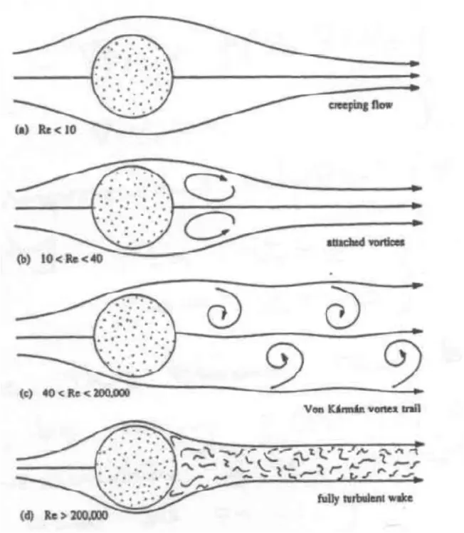
The Reynolds number(Re) is a dimensionless number used to categorize the fluids systems in which the effect of viscosity is important in controlling the velocities or the flow pattern of a fluid.

`Re = (rho* v*d)/mu`

Where `rho` = density

`v` = velocity

`d` = diameter

`mu` = viscosity

Process

We use Ansys Workbench here and chose Fluid Flow(Fluent).This is done in given steps.

Step-1 (Geometry) :-

• We draw a circle (of 2m dia) representing as a cylinder and draw a rectangle (of 62m x 20m) around it.
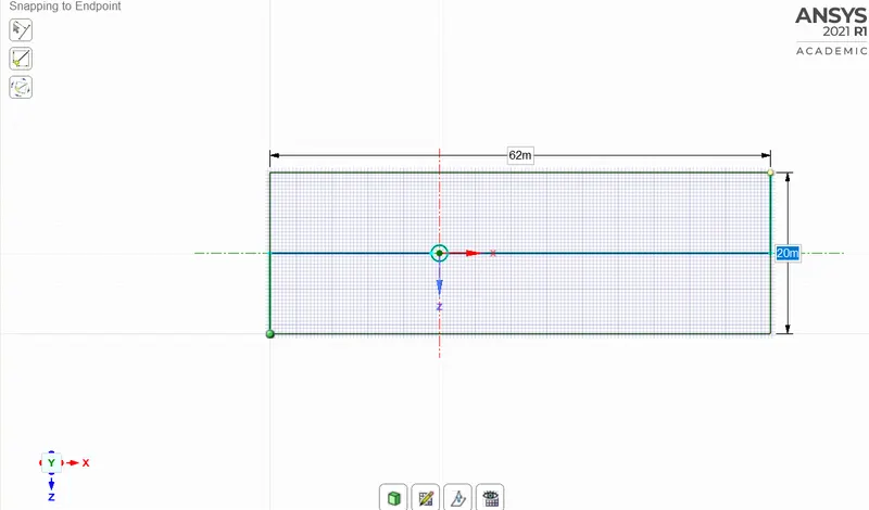
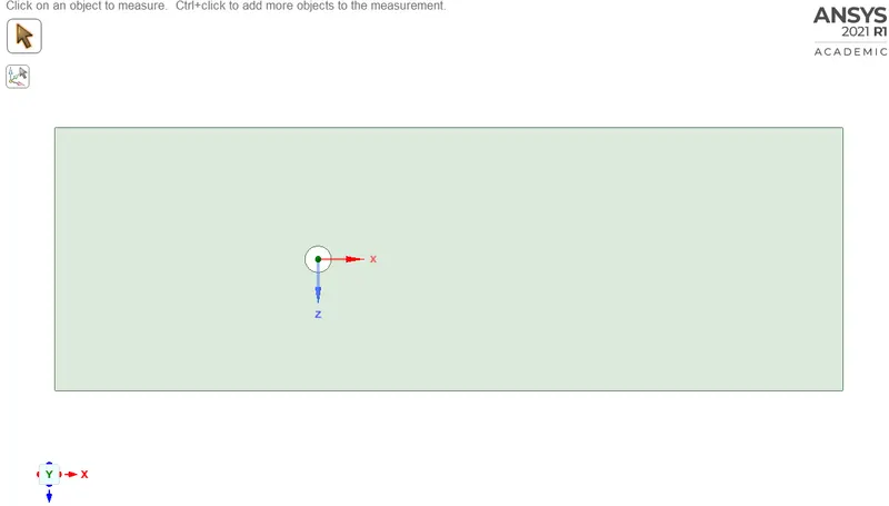
• Delete the circluler (cylinder) part by using pull tool.
• Delete all construction lines.

Step-2 (Meshing) :-

• Create Name Section(N) and name the boundries as inlet & outlet for top and bottom name it as symmetry and for cylinder circle name it as cylinder wall.
• Change the shape of the Mesh to trangular by inserting Method and set the element size at 0.25m.
• For a sharper circle insert Sizing and set the Number of Divisions to 36 which makes 360 view easy.
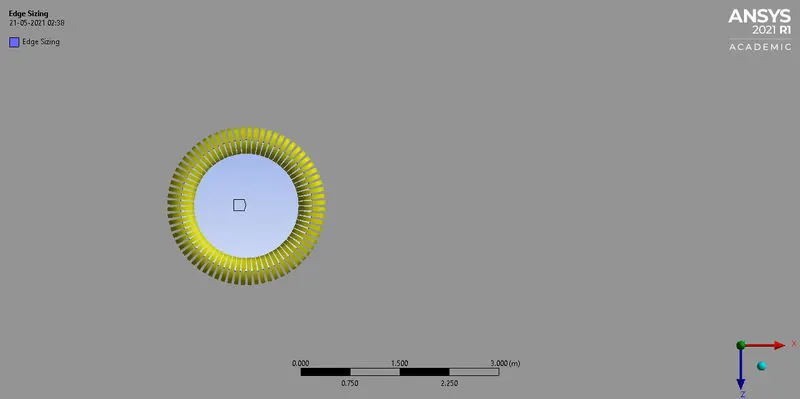
• To get more detailed results add multiple layers to the circle by inserting Inflation and setting the First layer Thickness to 5e-003m and Maxaimum Layers to 6.

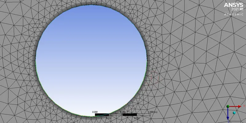
• Generate the Mesh

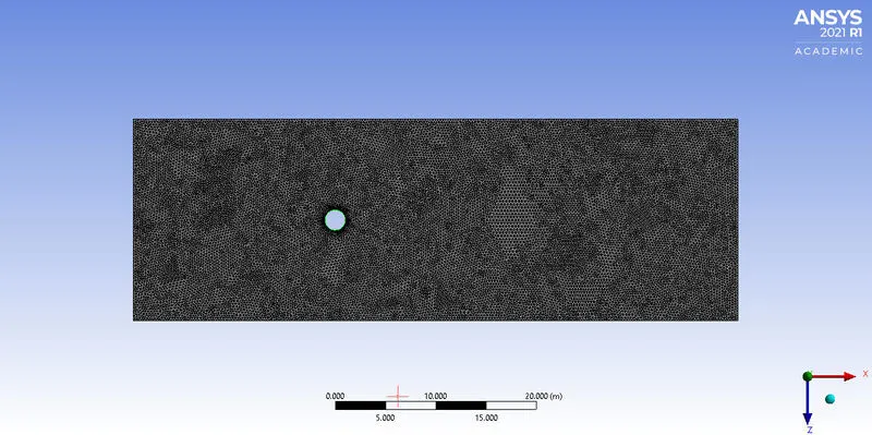
Step-3 (Setup) :-

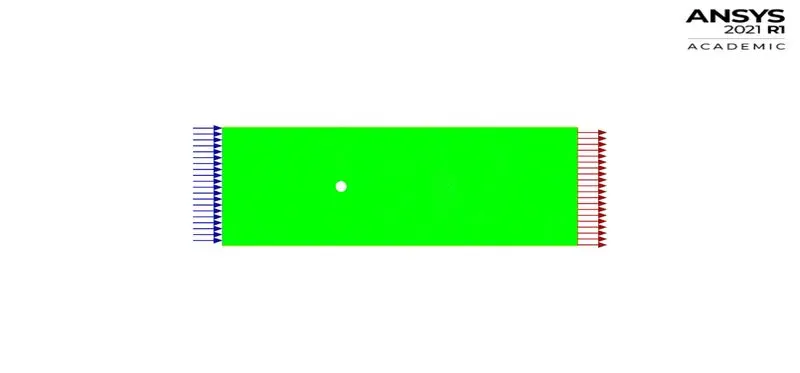
• Reference Values

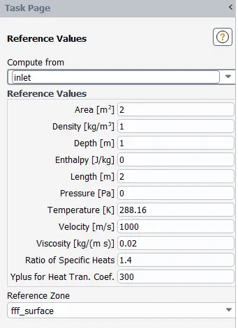
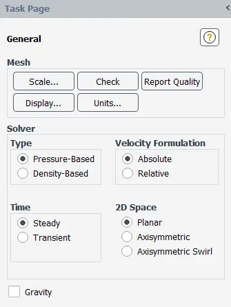
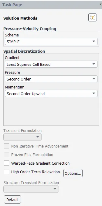
• General and Solution Method setting :- for Steady state we use SIMPLE Scheme and for Transient we use Coupled.

• Select Laminar in Viscous Model in Physics.
• To unselect air in Materials create new Fluent Fluid Materials and name it as user_material in Fluent Database.

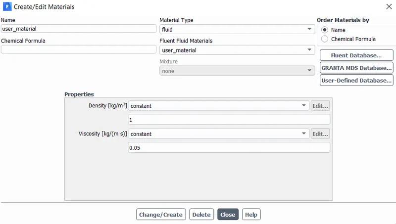
• Go to fff-surface in Cell Zones and change the material name to user_material and the delete the air from Fluent Fluid Materials.

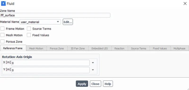
• Then in Material Properties for the user_material set the Density to 1 and change the Viscosity accordingly for different Reynolds number(Re) with steady solver.
• For Boundary conditions edit inlet Velocity to 1m/s and edit cylinder wall to No Slip.
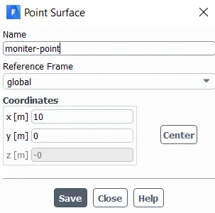
• Create Points for given cordinates name it as moniter-point or keep it as point-7.

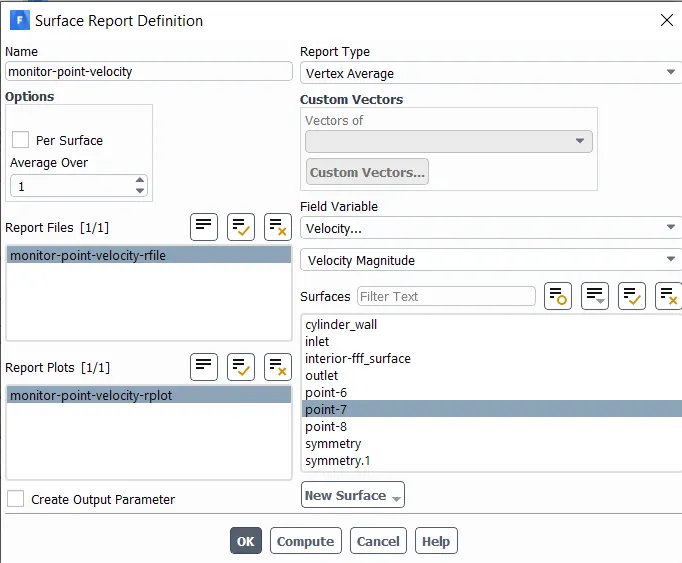
• Create a Surface Report at the given points and name it as moniter-point-velocity for type Vertex Average .

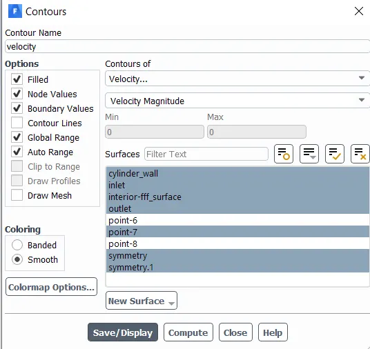
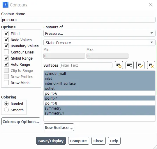
• Create Contour for Pressure and Velocity.

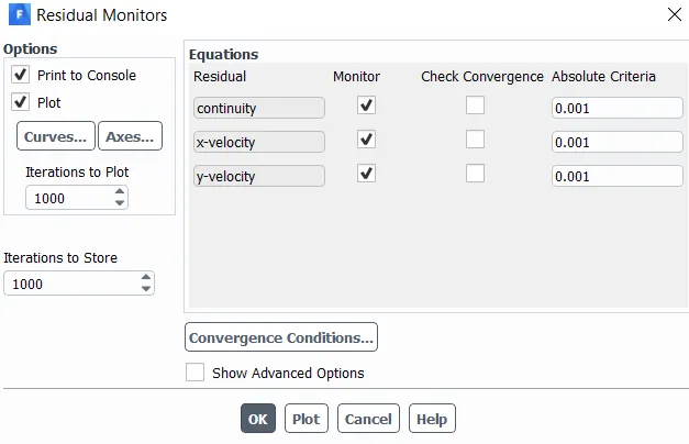
• Edit Residual Moniters
• In Force Reports create coefficient of drag and lift.
• Create solution Animations.

Simulation :- Running for 800 iterartions each case

Case-1 :-

Solution 1 :-

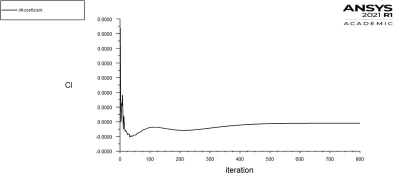
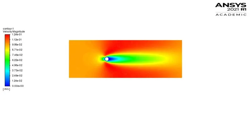
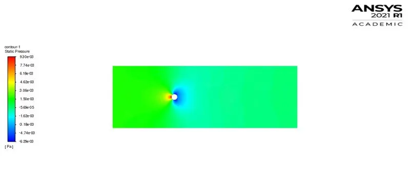
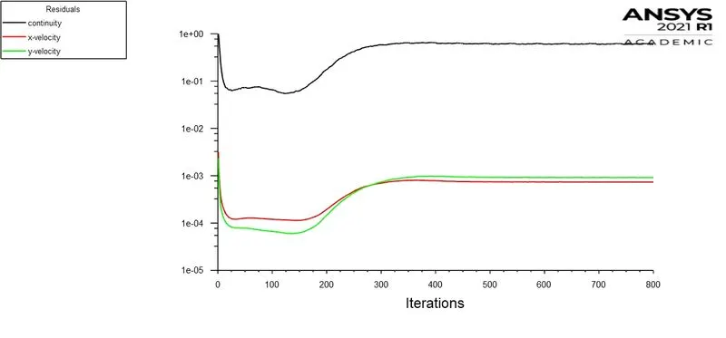
Reynolds number(Re) = 10

viscosity = 0.02 [kg/(m s)]

velocity = 0.1 (m/s)

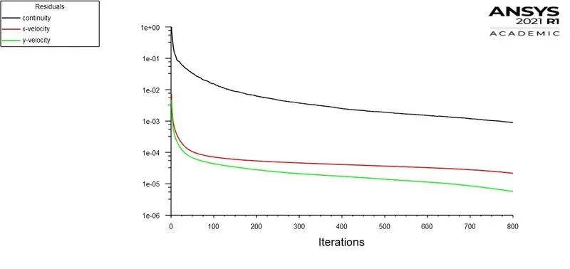
Residual Plot

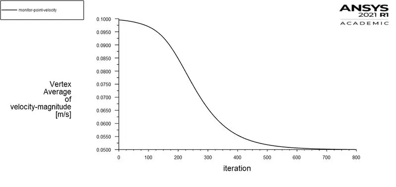
Vertex Average Plot

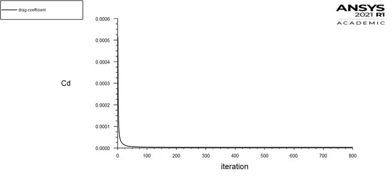
Drag Coefficient Plot

Lift Coefficient PLot

Velocity Contour

Pressure Contour

Solution 2 :-

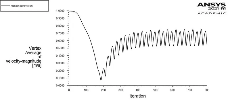
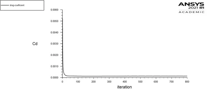
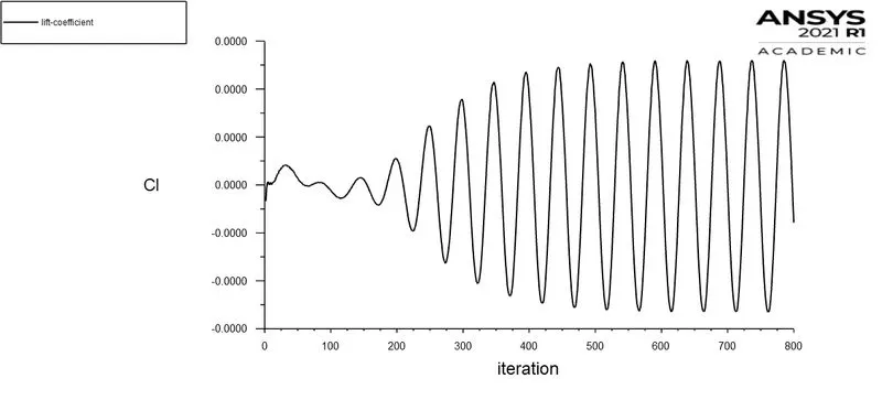
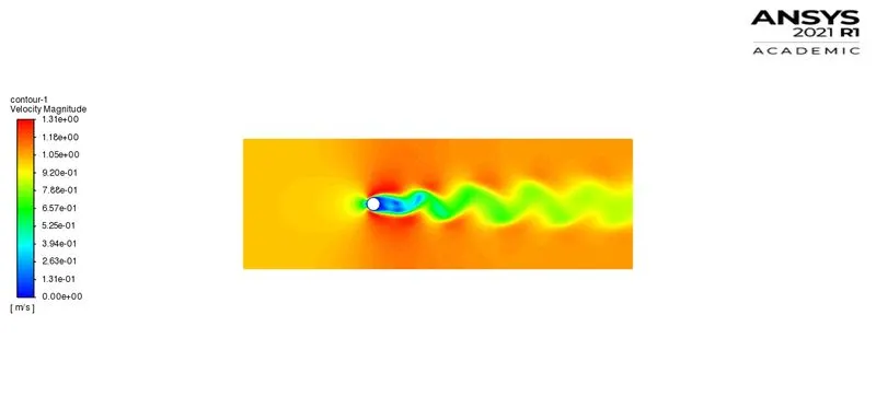
Reynolds number(Re) = 100

viscosity = 0.02 [kg/(m s)]

velocity = 1 (m/s)

Residual Plot

Vertex Average Plot

Drag Coefficient Plot

Lift Coefficient PLot

Velocity Contour

Pressure Contour

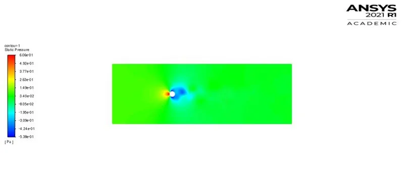
Solution 3 :- Transient state, For 3000 time steps,

Reynolds number(Re) = 100

viscosity = 0.02 [kg/(m s)]

velocity = 1 (m/s)

Residual Plot

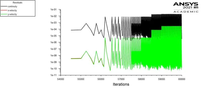
Vertex Average Plot

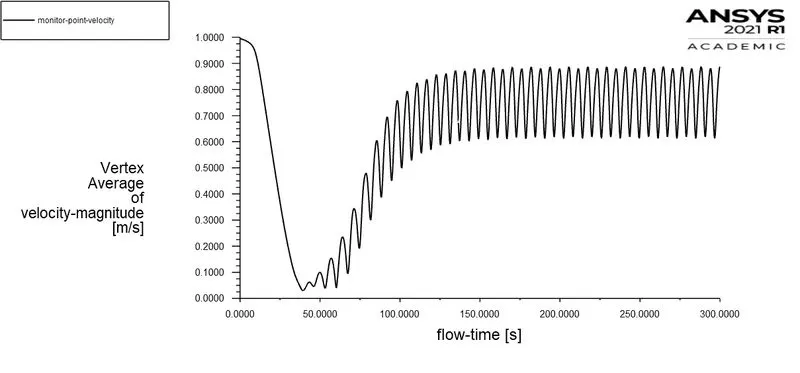
Drag Coefficient Plot

Lift Coefficient PLot

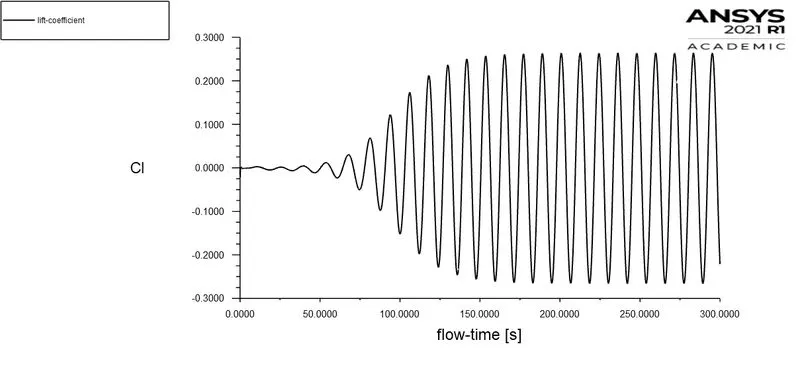
Velocity Contour

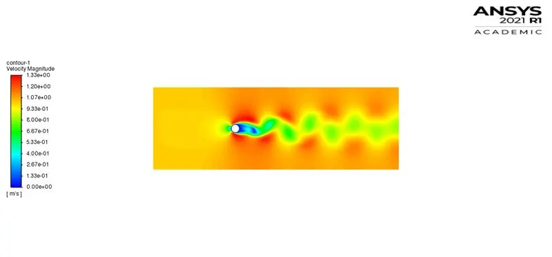
Pressure Contour

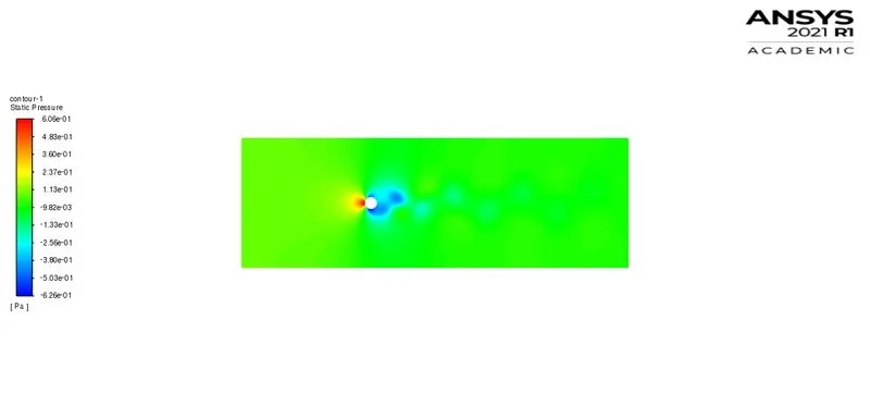
Strouhal Number :- It is a dimensionless number for flow fluctuation or instebility or which is describes oscillating flow mechanisms. It is an integral part of the fundamentals of fluid mechanics, given as

`St = (f*L)/v`

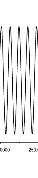
where `f` = frequency of vortex shedding = 4.3/(250-200) = 0.086 Hz -> value 4.3 is [approx] number of ossilations

This value is from Coefficient of Lift Plot -> value is -0.221

`L` = characteristic length = 2 m

`v` = fluid velocity = 1 m/s

It can only be calculated for unsteady state as it is time dependent and steady state is not.

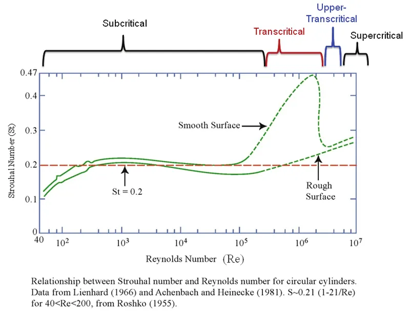
=> `St = (0.086*2)/1 = 0.172`

Case 2:-

Solution 4 :-

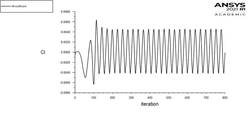
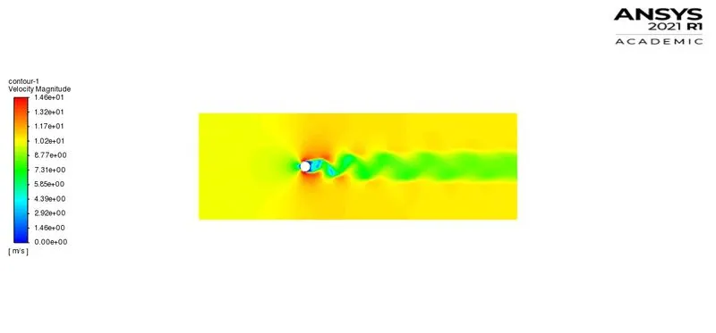
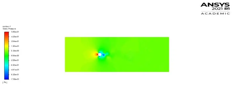
Reynolds number(Re) = 1000

viscosity = 0.02 [kg/(m s)]

velocity = 10 (m/s)

Residual Plot

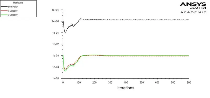
Vertex Average Plot

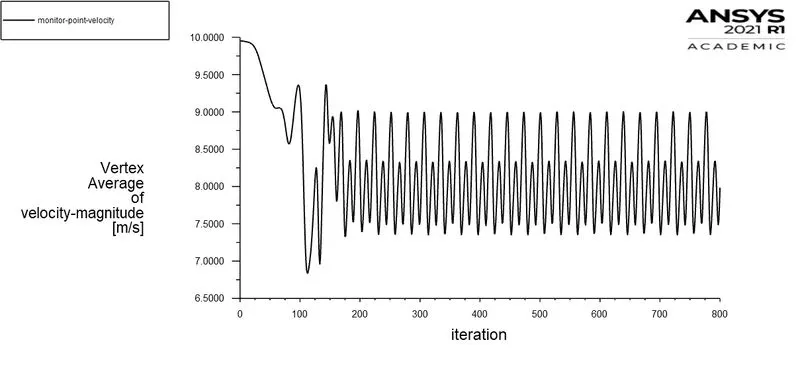
Drag Coefficient Plot

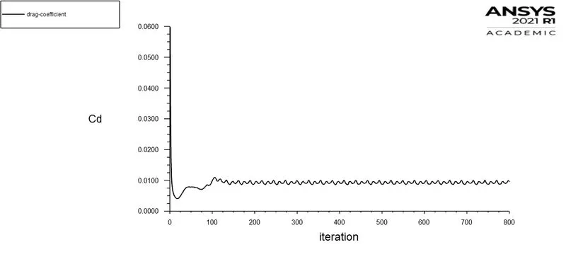
Lift Coefficient PLot

Velocity Contour

Pressure Contour

Solution 5 :-

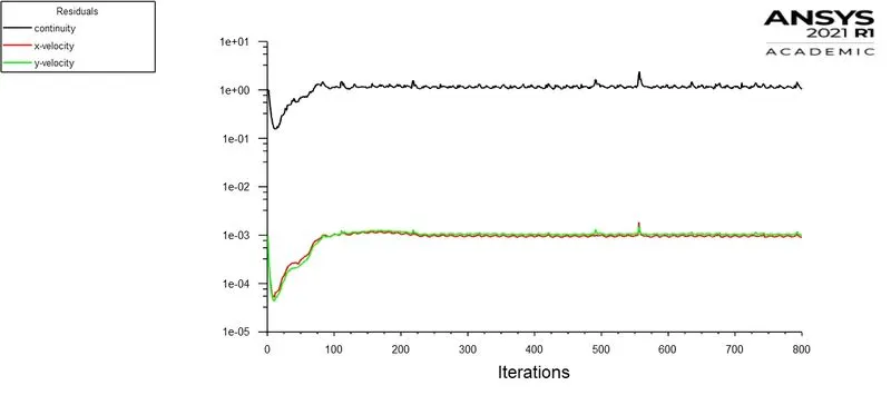
Reynolds number(Re) = 10000

viscosity = 0.02 [kg/(m s)]

velocity = 100 (m/s)

Residual Plot

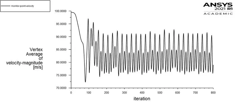
Vertex Average Plot

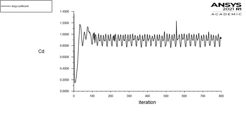
Drag Coefficient Plot

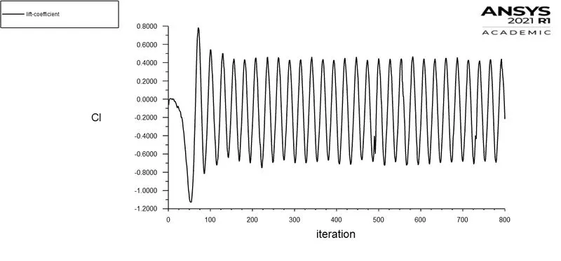
Lift Coefficient PLot

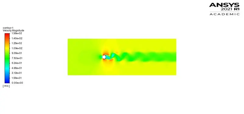
Velocity Contour

Pressure Contour

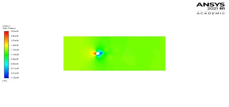
Solution 6 :-

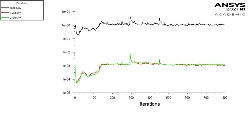
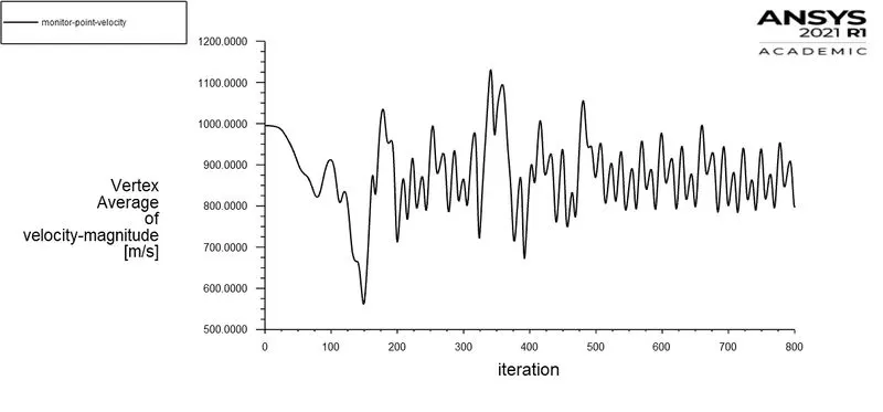
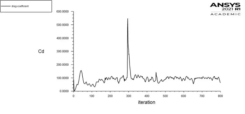
Reynolds number(Re) = 100000

viscosity = 0.02 [kg/(m s)]

velocity = 1000 (m/s)

Residual Plot

Vertex Average Plot

Drag Coefficient Plot

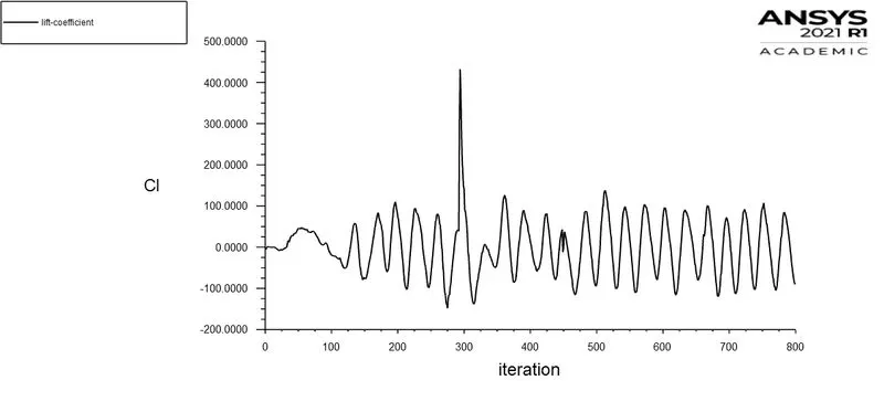
Lift Coefficient PLot

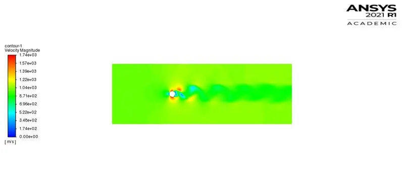
Velocity Contour

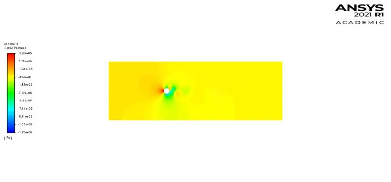
Pressure Contour

Results :-

State	Velovity (v)	Reynolds number(Re)	Coefficient of Drag (Cd)	Coefficient of Lift (Cl)
Steady	0.1	10	0.00000333	-1.89e-09
Steady	1	100	0.00013	-3.92e-06
Unsteady	1	100	1.397	-0.221
Steady	10	1000	0.0095	-0.0001
Steady	100	10000	0.915	-0.217
Steady	1000	100000	63.34	-87.4

Conclusion :-

When the Velocity (v) is low and when the Reynolds number (Re) is low then the Pressure (p) is more behind the cylinder and when (Re) is increased the pressure decreased behind the cylinder but the pressure at the front side remains same at any (Re) value. In laminar flow the (Re) value is below 10 the Flow stayes Steady and when it's around than 50 vertex shadding forms which are mostly symmetric and contra rotating formed behind the cylinder and when we increase (Re) value further the we will start losing symmentric form and at a certain value it will be completely lost and alternate side rotations will begin which will be around (Re) value 100. Around this the Vertex shading oscillation will be steady but as we go on increasing the (Re) value from 1000 to 10000 and furter more a disturbed type and not steady type (terbulent) vertex shadings oscillations are formed. And vertex shading oscillations also start forming early when the (Re) vale is increased. The sharp corners are formed in vertex shading behind the cylinder and they keep on increasing and get sharper with the increased (Re) value . In Coefficient of Lift (Cl) the number of oscillations for the given iterations keeps on increasing when we increase the (Re) value. Reynolds number (Re) effects Coefficient of Drag (Cd), from the above table as we increase (Re) value the (Cd) value also starts increasing and from the above plots for increased (Re) value the steadiness in (Cd) is lost and is disterbence is seen in it. In our Case we have added multiple layers and changed the first layer thickness for the better results. The material type we have used is user defined fluid where its Density is 1[kg/m^3] and its viscocity is 0.02 [kg/(m s)] . The Coefficient of Lift (Cl) in transient state the oscillations are larger in compared than steady state and Coefficient of Drag (Cd) is also larger in transient state than in steady state for the same (Re) value.