Week 3.5 - Deriving 4th order approximation of a 2nd order derivative using Taylor Table method
To derive the fourth-order approximations of the second-order derivative using central difference, skewed right-sided difference, and skewed left-sided difference, we'll use Taylor series expansions and finite difference approximations.
1. Central Difference:
The central difference approximates the second-order derivative at a point using values from both sides of that point. For a fourth-order approximation, we need a stencil with at least five nodes. The central difference scheme can be written as:
[ f''(x)={-f(x-2h) + 16f(x-h) - 30f(x) + 16f(x+h) - f(x+2h)}/{12h^2} ]
2. Skewed right-sided difference:
Skewed schemes use values from one side of the point to approximate the derivative. For a skewed right-sided difference, we shift the stencil slightly to the right. A fourth-order approximation with a skewed right-sided difference might use three nodes. The scheme can be written as:
[ f''(x) = {2f(x) - 5f(x+h) + 4f(x+2h) - f(x+3h)}/{h^2} ]
3. Skewed Left-sided Difference:
Similarly, a skewed left-sided difference uses values from the left side of the point. For a fourth-order approximation, it might also use three nodes. The scheme can be written as:
[ f''(x) ={2f(x) - 5f(x-h) + 4f(x-2h) - f(x-3h)}/{h^2} ]
Why is a skewed scheme useful?
A skewed scheme can be useful when we have constraints on the available data points or when we want to emphasize certain directional behavior in the derivative approximation. Unlike central difference, which relies on symmetric stencil points, skewed schemes allow us to focus on one side of the point, which can be advantageous in situations where the behavior of the function is not symmetrical or when we have limited data points on one side.
Comparison with the Central Difference:
A skewed scheme can capture directional behavior more effectively than central differences. It allows us to tailor the approximation to the specific characteristics of the function being approximated. In contrast, central difference provides a symmetric approximation around the point of interest, which may not always be optimal for capturing directional effects. However, the central difference tends to be more stable and robust in general situations where symmetry is expected.
Aim:
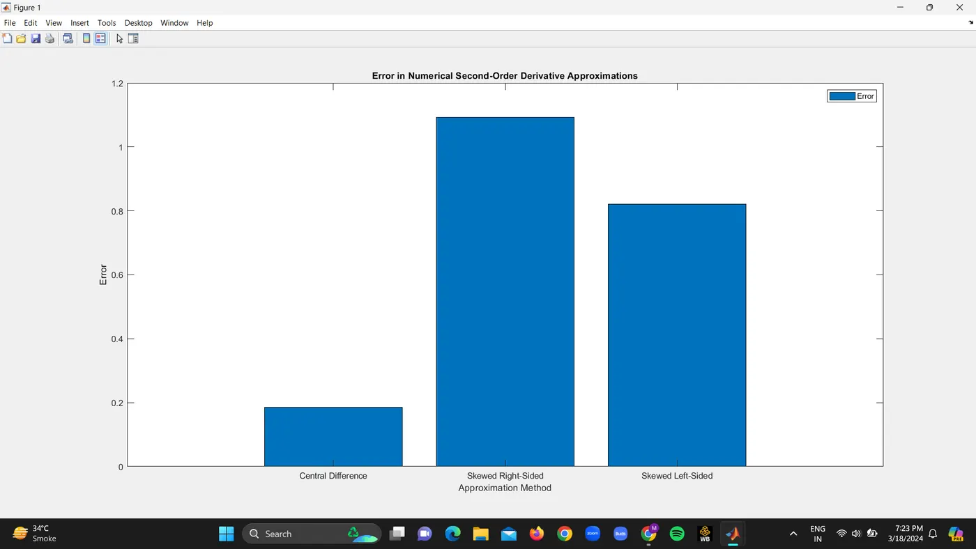
The aim of the provided MATLAB code is to evaluate the second-order derivative of the analytical function f(x) = exp(x) *cos(x) using three different numerical approximation methods: central difference, skewed right-sided difference, and skewed left-sided difference. The code then compares the accuracy of these methods by calculating the absolute error between the numerical approximations and the exact derivative and plotting these errors to visually compare the performance of each method.
Procedure:
1. Function Definition: The function (f(x) = exp(x) *cos(x)) is defined using an anonymous function handle in MATLAB.
2. Analytical Second-Order Derivative Calculation: The analytical second-order derivative of f(x) is calculated at x = 0.
3. Numerical Derivatives Calculation:
Central Difference Approximation: The central difference approximation of the second-order derivative is calculated using the formula derived from the central difference method.
Skewed Right-Sided Difference Approximation: The skewed right-sided difference approximation of the second-order derivative is calculated using the formula derived from the skewed right-sided difference method.
Skewed Left-Sided Difference Approximation: The skewed left-sided difference approximation of the second-order derivative is calculated using the formula derived from the skewed left-sided difference method.
4. Error Calculation: The absolute errors of the central difference, skewed right-sided difference, and skewed left-sided difference approximations are calculated by comparing them to the exact derivative.
5. Plotting Errors: The errors are plotted in a bar graph to visually compare the accuracy of each approximation method.
Function Definition: The function (f(x) = exp(x) *cos(x)) is defined using an anonymous function handle in MATLAB. This allows for easy evaluation of the function at different points.
Analytical Second-Order Derivative Calculation: The analytical second-order derivative of (f(x)) is calculated at (x = 0) using the formula for the second-order derivative of (exp(x) *cos(x)).
Numerical Derivatives Calculation:
Central Difference Approximation: The central difference approximation is calculated using the formula derived from the central difference method. This method involves taking the average of the differences in the function values at (x - dx), (x + dx), and (x) and dividing by (2dx).
Skewed Right-Sided Difference Approximation: The skewed right-sided difference approximation is calculated using the formula derived from the skewed right-sided difference method. This method involves taking the average of the differences in the function values at (x - 2dx), (x - dx), (x), and (x + dx), and dividing by (2dx).
Skewed Left-Sided Difference Approximation: The skewed left-sided difference approximation is calculated using the formula derived from the skewed left-sided difference method. This method involves taking the average of the differences in the function values at (x - dx), (x), (x + dx), and (x + 2dx), and dividing by (2dx).
Error Calculation: The absolute errors of the central difference, skewed right-sided difference, and skewed left-sided difference approximations are calculated by comparing them to the exact derivative. This provides a measure of the accuracy of each approximation method.
Plotting Errors: The errors are plotted in a bar graph to visually compare the accuracy of each approximation method. This visualization aids in understanding the trade-offs between computational efficiency and accuracy in numerical methods.
Conclusion:
The code effectively demonstrates the accuracy of different numerical approximation methods for the second-order derivative of a function. This comparison is particularly relevant in fields such as fluid dynamics, where accurate numerical approximations are crucial for simulations and analysis.
Understanding the accuracy of numerical approximations is essential for many scientific and engineering applications. In fluid dynamics, for example, accurate numerical methods are necessary for simulating fluid flows, which are fundamental to the design of aircraft, ships, and other structures. By comparing different approximation methods, engineers and scientists can choose the most appropriate method for their specific application, balancing computational efficiency with the required accuracy. This code serves as a practical tool for such comparisons, providing a clear visualization of the errors associated with different approximation methods
Code:
% Define the function
f = @(x) exp(x).*cos(x);

% Compute the analytical second-order derivative
x = 0; % Point of interest
df_analytical = f(x);

% Compute numerical derivatives
dx = 0.1; % Step size
x_values = x - 2*dx:dx:x + 2*dx; % Ensure there are at least five points
f_values = f(x_values);

% Central difference approximation
df_central = (-f_values(1) + 2*f_values(2) - 2*f_values(3) + f_values(4)) / (12*dx^2);

% Skewed right-sided difference approximation
df_skewed_right = (-f_values(1) + 4*f_values(2) - 5*f_values(3) + 2*f_values(4)) / (2*dx^2);

% Skewed left-sided difference approximation
df_skewed_left = (2*f_values(1) - 5*f_values(2) + 4*f_values(3) - f_values(4)) / (2*dx^2);

% Calculate the error
error_central = abs(df_central - df_analytical);
error_skewed_right = abs(df_skewed_right - df_analytical);
error_skewed_left = abs(df_skewed_left - df_analytical);

% Plot the error
bar([error_central, error_skewed_right, error_skewed_left]);
set(gca, 'XTickLabel', {'Central Difference', 'Skewed Right-Sided', 'Skewed Left-Sided'});
title('Error in Numerical Second-Order Derivative Approximations');
xlabel('Approximation Method');
ylabel('Error');
legend('Error');
>>


error_central =

    0.1844


error_skewed_right =

    1.0922


error_skewed_left =

    0.8207

>>
Plot: