Week 3.5 - Deriving 4th order approximation of a 2nd order derivative using Taylor Table method
Aim:
To derive the following 4th order approximations of second-order derivative.
1.Central difference
2.Skewed right-side difference
3.Skewed left-side difference
After deriving these schemes, prove that your skewed schemes are fourth-order accurate i.e the thumb rule given in Hint(2)
Once you have done this , Write a program in MATLAB to evaluate the second-order derivative of analytical function exp(x)*cos(x) and compare it with 3 numerical approximations that you have derived.
provide a plot that compares the absolute error between the above mention schemes.
In your own words, describe why skewed scheme is useful? What can a skewed do that CD scheme cannot?
Objective-1:Deriving the central, skwed right-side and skewed left-side differencing schemes.
1.4th order approximation of 2nd order Derivative using CENTRAL DIFFERENCING:
Number of nodes in CD=p+q-1
where p=order of derivative, q=order of approximation
- Number of nodes in CD=2+4-1=5,(i.e(i-2),(i-1),(i),(i+2),(i+1))
Hypothesis eqn
- (Δx^2)(∂^2f/∂x^2)=a.f(i-2)+b.f(i-1)+c.f(i)+d.f(i+1)+e.f(i+2)
Taylor series table
f(x) Δ(x).f'(x) Δx².f''(x) Δx³.f'''(x) Δx^4.f'4(x) Δx^5.f'5(x) Δx^6.f'6(x)
Δx^2(∂²f/∂x²)
a.f(i-2) a -2a 4a/2 -8a/6 16a/24 -32a/120 64a/720
b.f(i-1) b -b b/2 -b/6 b/24 -b/120 b/720
c.f(i) c 0 0 0 0 0 0
d.f(i+1) d d d/2 d/6 d/24 d/120 d/720
e.f(i+2) e 2e 4e/2 8e/6 16e/24 32e/120 64e/720
Δx²(∂²f/∂x²) 0 0 1 0 0 ? ?
Now the equation slove are
a+b+c+d+e=0
-2a-b+0+d+2e=0
2a+b/2+0+d/2+2e=1
-4a/3-b/6+0+d/6+4e/3=0
2a/3+b/24+0+d/24+2a/3=0
We will convert the above equation into matrix from
1 1 1 1 1 a 0
-2 -1 0 1 2 b 0
2 1/2 0 1/2 2 * c = 1
-4/3 -1/6 0 1/6 -4/3 d 0
2/3 1/24 0 1/24 2/3 e 0
The above matrix equation can be solved in MATLAB using linsolve() function,which is shown below
clear all
close all
clc
% PROGRAM TO SOLVE THE MATRIX EQUATION FORMED FOR CALCULATING THE CENTRAL
% DIFFERENCING SCHEME
A=[1,1,1,1,1;-2,-1,0,1,2;2,1/2,0,1/2,2;-4/3,-1/6,0,1/6,4/3;2/3,1/24,0,1/24,2/3]
B=[0;0;1;0;0]
C=A\B
→">
Output:
A =

    1.0000    1.0000    1.0000    1.0000    1.0000
   -2.0000   -1.0000         0    1.0000    2.0000
    2.0000    0.5000         0    0.5000    2.0000
   -1.3333   -0.1667         0    0.1667    1.3333
    0.6667    0.0417         0    0.0417    0.6667


B =

     0
     0
     1
     0
     0


C =

   -0.0833
    1.3333
   -2.5000
    1.3333
   -0.0833
Proof of Hypothesis function having a truncation error of order 4
Hence hypothesis function is
- (Δx^2)(∂^2f/∂x^2)=a.f(i-2)+b.f(i-1)+c.f(i)+d.f(i-1)+e.f(i+2)
- (Δx^2)(∂^2f/∂x^2)=a+b+c+d+e)f(x)+(-a-b+0+d+2e)(Δx)f'(x)+(2a+b/2+0+d/2+2e)(Δx²)f''(x)+(-4a/3-b/6+0+d/6+4e/3)(Δx³)f'''(x)+(2a/3+b/24+0+d/24+2a/3)(Δx^4)f''''(x)+(-4a/5-b/120+0+d/120+4e/5)(Δx^5)f'''''(x)+(4a/45+b/720+0+d/720+4e/45)(Δx^6)f''''''(x)
In the above equation, only the (Δx^2)and the Δx^6 term will be present, all other terms will become 0 if the coefficients are substituted.
(Δx^2)(∂^2f/∂x^2)=(2a+b/2+0+d/2+2e)(Δx²)f''(x)+(4a/45+b/720+0+d/720+4e/45)(Δx^6)f''''''(x)
(∂^2f/∂x^2)=(2a+b/2+d/2+2e)(Δx²)f''(x)+(4a/45+b/720+d/720+4e/45)(Δx^6)f"""(x)/(Δx²)
(∂^2f/∂x^2)=(2a+b/2+0+d/2+2e)f''(x)+(4a/45+b/720+0+d/720+4e/45)(Δx^4)f''''''(x)
The last term in above equation (i.e. trianglex^(4)) can be nehlected as truncation error.
(Δx^2)(∂^2f/∂x^2)=(2a+b/2+0+d/2+2e)(f''(x)+0(Δx^4)
Since the truncation error is of the order of 4, it is proved that the hypothesis function is for 4th order approximation.
Therefore, the hypothesis function for 4th order approximation using CENTRAL DIFFERENCING is
(∂^2f/∂x^2)=-0.0833.f(i-2)+1.3333.f(i-1)-2.5.f(i)+1.3333.f(i-1)-0.0833.f(i+2)/(Δx^2)
2.4th order Approximations of 2nd order Derivaive using SKWED RIGhT-SIDED DIFFERENCING SCHEME
Number of nodes in CD=p+q
where p=order of derivative, q=order of approximation
- Number of nodes in CD=2+4=6,(i.e(i),(i+1),(i+2),(i+3),(i+4),(i+5))
Hypothesis eqn
- (Δx^2)(∂^2f/∂x^2)=a.f(i)+b.f(i+1)+c.f(i+2)+d.f(i+3)+e.f(i+4)+g.f(i+5)
Taylor series table
f(x) Δ(x).f'(x) Δx².f''(x) Δx³.f'''(x) Δx^4.f'4(x) Δx^5.f'5(x) Δx^6.f'6(x)
Δx^2(∂²f/∂x²)
a.f(i) a 0 0 0 0 0 0
b.f(i+1) b b b/2 b/6 b/24 b/120 b/720
c.f(i+2) c 2c 4c/2 8c/6 16c/24 32c/120 64c/720
d.f(i+3) d 3d 9d/2 27 d/6 81d/24 243d/120 729 d/720
e.f(i+4) e 4e 16e/2 64e/6 256e/24 1024e/120 4096e/720
g.f(i+5) g 5g 25g/2 125e/6 625g/24 3125g/120 15625g/720
Δx²(∂²f/∂x²) 0 0 1 0 0 ? ?
Now the equations to solve are
a+b+c+d+e+g=0
0+b+2c+3d+4e+5g=0
0+b/2+4c/2+9d/2+16e/2+25g/2=1
0+b/6+8c/6+27d/6+64e/6+125e/6=0
0+b/24+16c/24+81d/24+256e/24+625g/24=0
0+b/120+32c/120+243d/120+1024e/120+3125g/120=0
We will convert the above equation into matrix from
1 1 1 1 1 1 a 0
0 1 2 3 4 5 b 0
0 1/2 4/2 9/2 16/2 25/2 * c = 1
0 1/6 8/6 27/6 64/6 125/6 d 0
0 1/24 16/24 81/24 256/24 625/24 e 0
0 1/24 32/120 243/120 1024/120 3125/120 g 0
The above matrix equation can be solved in MATLAB using linsolve() function,which is shown below
clear all
close all
clc

A=[1 1 1 1 1 1;
    0,1,2,3,4,5;
    0,1/2,2,9/2,8,25/2;
    0 1/6 8/6 27/6 64/6 125/6;
    0,1/24,16/24,81/24,256/24,625/24;
    0 1/120 32/120 243/120 1024/120 3125/120]
B=[0;0;1;0;0;0]
c=linsolve(A,B)
A =
1.0000 1.0000 1.0000 1.0000 1.0000 1.0000
0 1.0000 2.0000 3.0000 4.0000 5.0000
0 0.5000 2.0000 4.5000 8.0000 12.5000
0 0.1667 1.3333 4.5000 10.6667 20.8333
0 0.0417 0.6667 3.3750 10.6667 26.0417
0 0.0083 0.2667 2.0250 8.5333 26.0417
B =
0
0
1
0
0
0
c =
3.7500
-12.8333
17.8333
-13.0000
5.0833
-0.8333Therefore, the hypothesis function for 4th order approximation using SkEWED RIGHT- SIDE DIFFERENCING is
(∂^2f/∂x^2)=3.75.f(i)-12.833.f(i+1)+17.8333.f(i+2)-13.f(i+3)+5.0833.f(i+4)-0.833.f(i+5)/(Δx^2)
3.4th order Approximations of 2nd order Derivaive using SKWED LEFT-SIDED DIFFERENCING SCHEME
Number of nodes in CD=p+q
where p=order of derivative, q=order of approximation
- Number of nodes in CD=2+4=6,(i.e(i),(i-1),(i-2),(i-3),(i-4),(i-5))
Hypothesis eqn
- (Δx^2)(∂^2f/∂x^2)=a.f(i)+b.f(i-1)+c.f(i-2)+d.f(i-3)+e.f(i-4)+g.f(i-5)
Taylor series table
f(x) Δ(x).f'(x) Δx².f''(x) Δx³.f'''(x) Δx^4.f'4(x) Δx^5.f'5(x) Δx^6.f'6(x)
Δx^2(∂²f/∂x²)
a.f(i) a 0 0 0 0 0 0
b.f(i+1) b - b b/2 - b/6 b/24 - b/120 b/720
c.f(i+2) c -2c 4c/2 - 8c/6 16c/24 -32c/120 64c/720
d.f(i+3) d -3d 9d/2 -27 d/6 81d/24 -243d/120 729 d/720
e.f(i+4) e - 4e 16e/2 -64e/6 256e/24 -1024e/120 4096e/720
g.f(i+5) g -5g 25g/2 -125e/6 625g/24 -3125g/120 15625g/720
Δx²(∂²f/∂x²) 0 0 1 0 0 ? ?
Now the equations to solve are
a+b+c+d+e+g=0
0-b-2c-3d-4e-5g=0
0+b/2+4c/2+9d/2+16e/2+25g/2=1
0-b/6-8c/6-27d/6-64e/6-125e/6=0
0+b/24+16c/24+81d/24+256e/24+625g/24=0
0-b/120-32c/120-243d/120-1024e/120-3125g/120=0
We will convert the above equation into matrix from
1 1 1 1 1 1 a 0
0 -1 - 2 -3 - 4 -5 b 0
0 1/2 4/2 9/2 16/2 25/2 * c = 1
0 -1/6 -8/6 -27/6 -64/6 -125/6 d 0
0 1/24 16/24 81/24 256/24 625/24 e 0
0 -1/24 -32/120 -243/120 -1024/120 -3125/120 g 0
clear all
close all
clc

A=[1 1 1 1 1 1;
    0,-1,-2,-3,-4,-5;
    0,1/2,2,9/2,8,25/2;
    0,-1/6 -8/6 -27/6 -64/6 -125/6;
    0,1/24,16/24,81/24,256/24,625/24;
    0 -1/120 -32/120 -243/120 -1024/120 -3125/120]
B=[0;0;1;0;0;0]
c=linsolve(A,B)
A =
Columns 1 through 4
1.0000 1.0000 1.0000 1.0000
0 -1.0000 -2.0000 -3.0000
0 0.5000 2.0000 4.5000
0 -0.1667 -1.3333 -4.5000
0 0.0417 0.6667 3.3750
0 -0.0083 -0.2667 -2.0250
Columns 5 through 6
1.0000 1.0000
-4.0000 -5.0000
8.0000 12.5000
-10.6667 -20.8333
10.6667 26.0417
-8.5333 -26.0417
B =
0
0
1
0
0
0
c =
3.7500
-12.8333
17.8333
-13.0000
5.0833
-0.8333Therefore, the hypothesis function for 4th order approximation using SkEWED LEFT- SIDE DIFFERENCING is
(∂^2f/∂x^2)=3.75.f(i)-12.833.f(i+1)+17.8333.f(i+2)-13.f(i+3)+5.0833.f(i+4)-0.833.f(i+5)/(Δx^2)
Objective -2
Write a program in MATLAB toevaluate the second-order derivative of the analytical function exp(x)*cos(x) and compare it with the 3 numerical approximations that you have derived. Provide a plot that compares the absolute error between the above-mentioned schemes
% Clear the workspace, close all figures, and clear the command window
clear all
close all
clc
% Set the value of x, range of dx values, and define the function and its analytical derivative
x=pi/3
dx=linspace(pi/4000,pi/40,200)
f=@(x) exp(x)*cos(x)

analytical_derivative=-2*exp(x)*sin(x)
%Coefficient matrices for central differencing
A=[1,1,1,1,1;-2,-1,0,1,2;2,1/2,0,1/2,2;-4/3,-1/6,0,1/6,4/3;2/3,1/24,0,1/24,2/3]
B=[0;0;1;0;0]
x_c=A\B
% Coefficient matrices for right-skewed differencing
A=[1 1 1 1 1 1;0,1,2,3,4,5;0,1/2,2,9/2,8,25/2;0 1/6 8/6 27/6 64/6 125/6;0,1/24,16/24,81/24,256/24,625/24;
    0 1/120 32/120 243/120 1024/120 3125/120]
B=[0;0;1;0;0;0]
x_r=linsolve(A,B)
% Coefficient matrices for left-skewed differencing
A=[1 1 1 1 1 1;0,-1,-2,-3,-4,-5;0,1/2,2,9/2,8,25/2;0,-1/6 -8/6 -27/6 -64/6 -125/6;0,1/24,16/24,81/24,256/24,625/24;
    0 -1/120 -32/120 -243/120 -1024/120 -3125/120]
B=[0;0;1;0;0;0]
x_l=linsolve(A,B)
% Initialize arrays for errors
central_differencing_error=zeros(size(dx))
right_skewed_error = zeros(size(dx))
left_skewed_error = zeros(size(dx))
% Loop over dx values to calculate finite difference approximations and errors
for i=1:length(dx)
    % Central differencing
    central_differencing(i)=x_c(1)*f(x-2*dx(i))+x_c(2)*f(x-dx(i))+x_c(3)*f(x)+x_c(4)*f(x+dx(i))+x_c(5)*f(x+2*dx(i));
     % Right-skewed differencing
    skewed_right_differencing(i)=x_r(1)*f(x)+x_r(2)*f(x+dx(i))+x_r(3)*f(x+2*dx(i))+x_r(4)*f(x+3*dx(i))+x_r(5)*f(x+4*dx(i))+x_r(6)*f(x+5*dx(i));
     % Left-skewed differencing
    skewed_left_differencing(i)=x_l(1)*f(x)+x_l(2)*f(x-dx(i))+x_l(3)*f(x-2*dx(i))+x_l(4)*f(x-3*dx(i))+x_l(5)*f(x-4*dx(i))+x_l(6)*f(x-5*dx(i));
    % Compute absolute errors
    central_differencing_error(i)=abs(central_differencing(i)/dx(i)^2-analytical_derivative)
    right_skewed_error(i)=abs(skewed_right_differencing(i)/dx(i)^2-analytical_derivative)
    left_skewed_error(i)=abs(skewed_left_differencing(i)/dx(i)^2-analytical_derivative)

end

% Plot errors on a log-log scale
loglog(dx,left_skewed_error,'y')
hold on
loglog(dx,central_differencing_error,'b')
loglog(dx,right_skewed_error,'color','r')
xlabel('log dx')
ylabel('log Error')
title("Error for numerical Approximation for dx value for 200 number's ranging from pi/4000 to pi/40 ")
legend("left skewed scheme","central differencing scheme","right skewed scheme")

%Slope of the curve obtained

slope_of_left_skewed_scheme = mean(diff(log(left_skewed_error))./diff(log(dx)))
slope_of_central_differencing_scheme = mean(diff(log(central_differencing_error))./diff(log(dx)))
slope_of_right_skewed_scheme = mean(diff(log(right_skewed_error))./diff(log(dx)))
Explanation:
- Initialize the workspace by clearing varibles,closeing figures, and clearing the command eindow.
- It is set up values of x and a range of dx values.
- Defines the function f(x)=exp(x)*cos(x) and computes the analytical derivative at the given point.
- This section defines coefficient matrices for the finite difference schemes:centeral differencing,right-skewed differencing, and left-skewed differencing.
- The matrices are used to calculate the coefficient x_c,x_r andx_l by solving linear systems.
- Initializes arrays to store the errors for each finite difference scheme.
- This loop calculates the finite difference approximations and error for each scheme using the specified dx values.
- Plots the errors on a log-log sclaes tovisualize error.
- Calculate the slopes.
output:
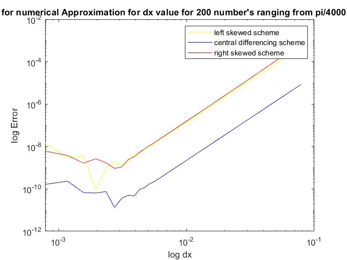
The comparison of absolute error for the left, right and central differencing scheme can be seen in the below graph. The graph shows that the central scheme is most accurate compared to skewed differencing. The curves also shows that when the value of dx is very small or large the approximating function becomes unstabel. This instability is caused due to the combination of various errors such as roundoff error, residual error and truncation error.
A skewed scheme is useful when we have to predict using the boundary condition as we have only one direction to go. Hence the skewed scheme will be useful and we cannot use the central differencing scheme for such an application because it required information from both direction of the point.