Week 3.5 - Deriving 4th order approximation of a 2nd order derivative using Taylor Table method

Aim:

The main aim of the challenge is to derive the 4th order approximations of the second-order derivative.

1. Central difference

2. Skewed right-sided difference

3. Skewed left-sided difference

Objective:

The objective of the project is to,

1. To calculate the second order derivative of the function f(x) = sin(x)*cos(x) using Central difference, Skewed right-sided difference, Skewed left-sided difference.
2. To plot and evaluate the results of the three approaches' results and errors.

Theory and derivations:

We might come across a partial derivative equation with a second order derivative when solving a CFD problem. Since we might have to choose a numerical technique rather than an analytical one due to the complexity of the problem. However, while using a numerical technique, we want to minimize the error margin.

We get increasing precision as the order of approximation increases. As a result, we'll come up with three ways to approximate an analytical function. The steps are as follows.

Central difference:

The nodes chosen in this case are symmetrical, indicating that the data comes from both sides of the point of focus. Using Taylor's approach, we obtain two nodes taken from both sides of the point of focus.

`(del^2f)/(delx^2) = s f(i-2) + b f(i-1) - c f(i) + d f(i+1) + e f(i+2)`

HINT given , For symmertical or central differencing N = p + q - 1

Taylor’s table for Central difference:

	f(x)	dx f'(x)	dx2 f''(x)	dx3 f'''(x)	dx4 f''''(x)	dx5 f'''''(x)
a f(i-2)	a	-2a	b/2	-8a/6	16a/24	-32a/120
b f(i-1)	b	-b	b/2	-b/6	b/24	-b/120
c f(i)	c	0	0	0	0	0
d f(i+1)	d	d	d/2	d/6	d/24	d/120
e f(i+2)	e	2e	4e/2	8e/6	16e/24	32e/120
a f(i-2) + b f(i-1) - c f(i) + d f(i+1) + e f(i+2)	0	0	1	0	0

This table transform into matrix of type AX=B

i.e. Values = a = -0.0833 b= 1.3333 c= -2.5000 d= 1.3333 e= -0.0833

These coefficients will subsequently be employed in the code to calculate the derivative value.

Skewed right-sided difference: In instances of initial boundary conditions where data points from the left nodes are unavailable, it becomes necessary to depend on the existing dataset for calculations.

Taylor’s table for Skewed right sided difference:

	f(x)	dx f’ (X)	dx2 f’’ (x)	dx3 f’’’(x)	dx4f’’’’(x)	dx5f’’’’’(x)
af(i)	a	0	0	0	0	0
bf(i+1)	b	b	b/2	b/6	b/24	b/120
cf(i+2)	c	2c	4c/2	8c/6	16c/24	32c/120
df(i+3)	d	3d	9d/2	27d/6	81d/24	243d/120
ef(i+4)	e	4e	16e/2	64e/6	256e/24	1024e/120
ff(i+5)	f	5f	25f/2	125f/6	625f/24	3125f/120
af(i) + bf(i+1) + cf(i+2) + df(i+3) + ef(i+4) +ff(i+5)	0	0	1	0	0	0

This table transform into matrix of type AX=B:[1111110123450122921622520168627664612560124162481242562462524011203212024312010241203125120]".

unknown i.e. Values = a = 3.7500 b= -12.8333 c= 17.8333

d= -13.0000 e= 5.0833 f= -0.8333

These coefficients will subsequently be employed in the code to calculate the derivative value.

Skewed left sided difference:

In cases of boundary conditions where data points from the right nodes are unavailable, reliance on the available dataset becomes necessary for calculations.

Taylor’s table for Skewed right sided difference:

	f(x)	dx f’ (X)	dx2 f’’ (x)	dx3 f’’’(x)	dx4f’’’’(x)	dx5f’’’’’(x)
af(i-5)	a	-5a	25a/2	-125a/6	625a/24	-3125a/120
bf(i-4)	b	-4b	16b/2	-64b/6	256b/24	-1024b/120
cf(i-3)	c	-3c	9c/2	-27c/6	81c/24	-243c/120
df(i-2)	d	-2d	4d/2	-8d/6	16d/24	-32d/120
ef(i-1)	e	-e	e/2	-e/6	e/24	-e/120
ff(i)	f	0	0	0	0	0
af(i-5) + bf(i-4) + cf(i-3) + df(i-2) + ef(i-1) +ff(i)	0	0	1	0	0

This table transform into matrix of type AX=B:

unknown i.e. Values = a = -0.8333 b= 5.0833 c=13.0000

d= 17.8333 e= -12.8333 f= 3.7500

These coefficients will subsequently be employed in the code to calculate the derivative value.

Matlab code:

clear all
close all
clc

%analytical function defination and value assignment
x=pi/3;
dx=linspace(pi/10,pi/1000,100);
f=@(x)(exp(x)*cos(x));
g=@(x)(-2*exp(x)*sin(x));
d2f=g(x);
func=f(x);



%for central difference scheme 
%coefficients taken from taylor's table
P = [1 1 1 1 1
    -2 -1 0 1 2
    4/2 1/2 0 1/2 4/2
    -8/6 -1/6 0 1/6 8/6
    16/24 1/24 0 1/24 16/24];
    
   
    
    
C=[0;0;1;0;0];
%as P*a=C i.e. a=inverse(P)*c(fastest way to getby '\')

cf1=P\C;

%for right skewwd differnce scheme
Q= [1 1 1 1 1 1
    0 1 2 3 4 5
    0 1/2 2 9/2 16/2 25/2
    0 1/6 8/6 27/6 64/6 125/6
    0 1/24 16/24 81/24 256/24 625/24
    0 1/120 32/120 243/120 1024/120 3125/120];
D=[0;0;1;0;0;0];
%as Q*b=s i.e. b=inverse(Q)*s(fastest way to getby '\')

cf2=Q\D;

%for right skewwd differnce scheme
R= [1 1 1 1 1 1
    -5 -4 -3 -2 -1 0
    25/2 16/2 9/2 2 1/2 0
    -125/6 -64/6 -27/6 -8/6 -1/6 0
    625/24 256/24 81/24 16/24 1/24 0
    -3125/120 -1024/120 -243/120 -32/120 -1/120 0];
E=[0;0;1;0;0;0];
%as n*b=s i.e. b=inverse(n)*s(fastest way to getby '\')

cf3=R\E;

%calculating values of derivative using CDS RSDC,LSDC
%defining variable size befor using in loop
central_diff=zeros(1,100);
err_central=zeros(1,100);
right_sdiff=zeros(1,100);
err_right=zeros(1,100);
left_sdiff=zeros(1,100);
err_left=zeros(1,100);

for i=1:length(dx)
    %calculating value and error by central difference scheme
    central_diff(i)=(cf1(1)*f(x-2*dx(i))+cf1(2)*f(x-dx(i))+cf1(3)*f(x)+cf1(4)*f(x+dx(i))+cf1(5)*f(x+2*dx(i)))/(dx(i))^2;
    err_central(i)=abs(central_diff(i)-d2f);
    
    %calculating value and error by right skewed difference scheme
    right_sdiff(i)=(cf2(1)*f(x)+cf2(2)*f(x+dx(i))+cf2(3)*f(x+2*dx(i))+cf2(4)*f(x+3*dx(i))+cf2(5)*f(x+4*dx(i))+cf2(6)*f(x+5*dx(i)))/(dx(i))^2;
    err_right(i)=abs(right_sdiff(i)-d2f);
    
    %calculating value and error by left skewed difference scheme
   left_sdiff(i)=(cf3(1)*f(x-5*dx(i))+cf3(2)*f(x-4*dx(i))+cf3(3)*f(x-3*dx(i))+cf3(4)*f(x-2*dx(i))+cf3(5)*f(x-dx(i))+cf3(6)*f(x))/(dx(i))^2;
   err_left(i)=abs(left_sdiff(i)-d2f); 

end

%plotting values of derivative
subplot(2,1,1)
hold on
fplot(d2f,'--')

xlim([-0.05 0.35]);
plot(dx,central_diff,'linewidth',2,'color','r');
plot(dx,right_sdiff,'linewidth',2,'color','b');
plot(dx,left_sdiff,'linewidth',2,'color','g');
legend('analytical value at x=pi/3','central diff.','right skewed diff.','left skewed diff.','location','best')
xlabel('Grid siza(dx)');
ylabel('Value');
title('Comparision b\w value of derivative calculated by diff. order of approximation') 
hold off

%plotting errors in approximation of derivative
subplot(2,1,2)
loglog(dx,err_central,'linewidth',2,'color','r');
hold on
xlim([.002 0.4]);
loglog(dx,err_right,'linewidth',2,'color','b');
loglog(dx,err_left,'linewidth',2,'color','g');
legend('central diff.','right skewed diff.','left skewed diff.','location','best')
xlabel('Grid siza(dx)');
ylabel('Absolute error');
title('Comparision b/w 4th order approximation method for error in calculating d2f/dx2 ');

Explanation:

1. Begin by setting the value of x and establishing the range of dx.
2. Create an anonymous function for a logical operation and its outcome.
3. Utilize matrices from the previously discussed section and solve the system through inversion, i.e., layoff = B => X = A⁻¹B.
4. Save the resulting components as cf1, cf2, and cf3.
5. Assign appropriate rows and columns to corresponding matrices.
6. Employ a for loop to iterate through the order of approximation expressions within the dx range. Additionally, compute the absolute error by comparing the calculated values to secondary values obtained analytically.
7. Collate the calculated values for a more effective compariso

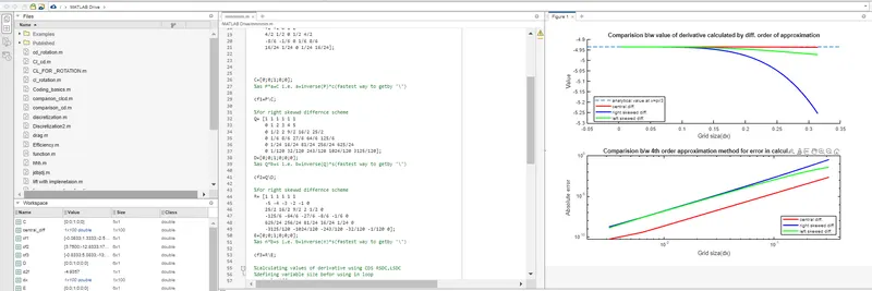
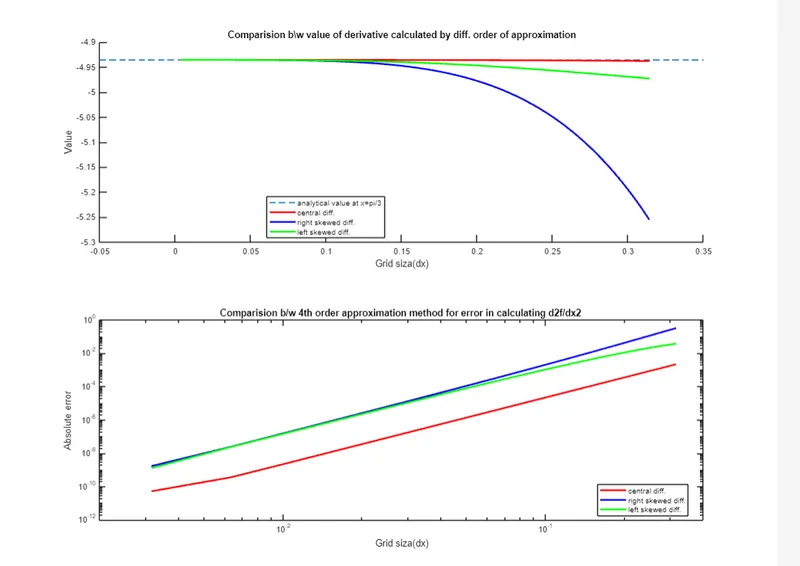
1. In the initial plot, an evident trend emerges as the size of dx decreases—each approximation converges toward the analytically computed value.

2. Upon observing the second plot, a notable pattern becomes apparent: the error associated with the central difference method is notably smaller when contrasted with the other two method.