Week 3.5 - Deriving 4th order approximation of a 2nd order derivative using Taylor Table method
Aim:
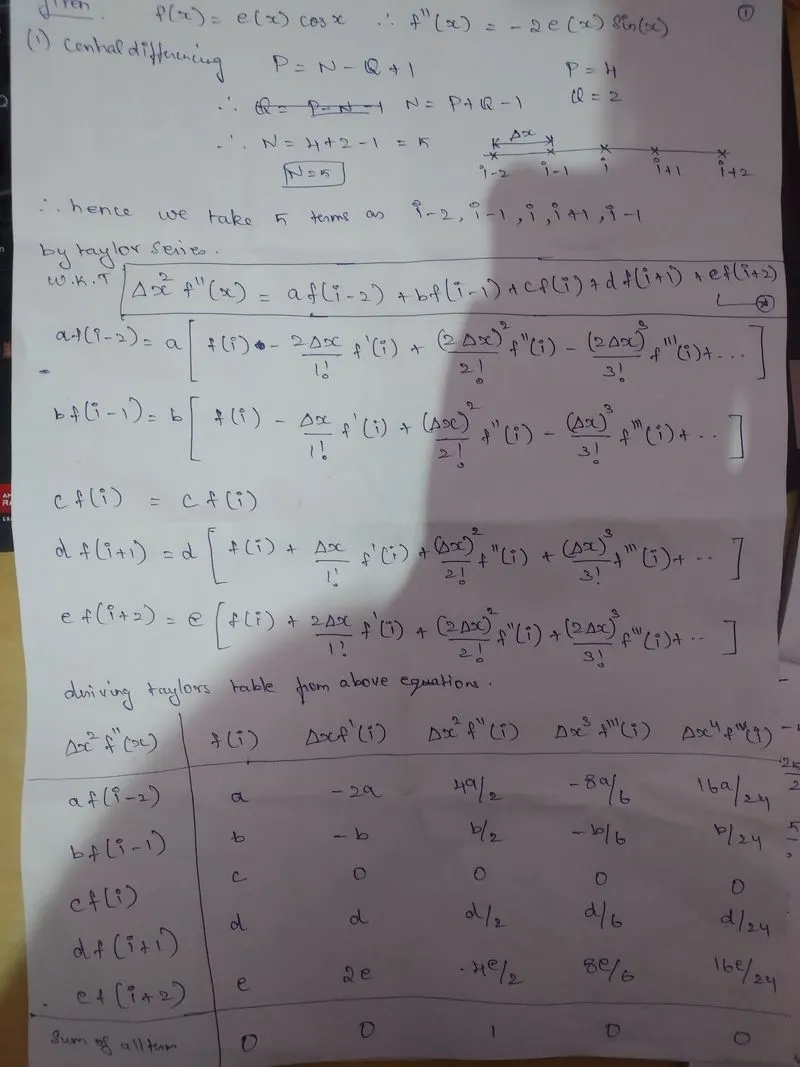
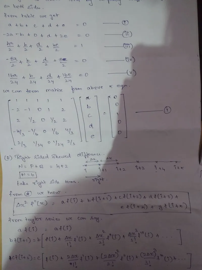
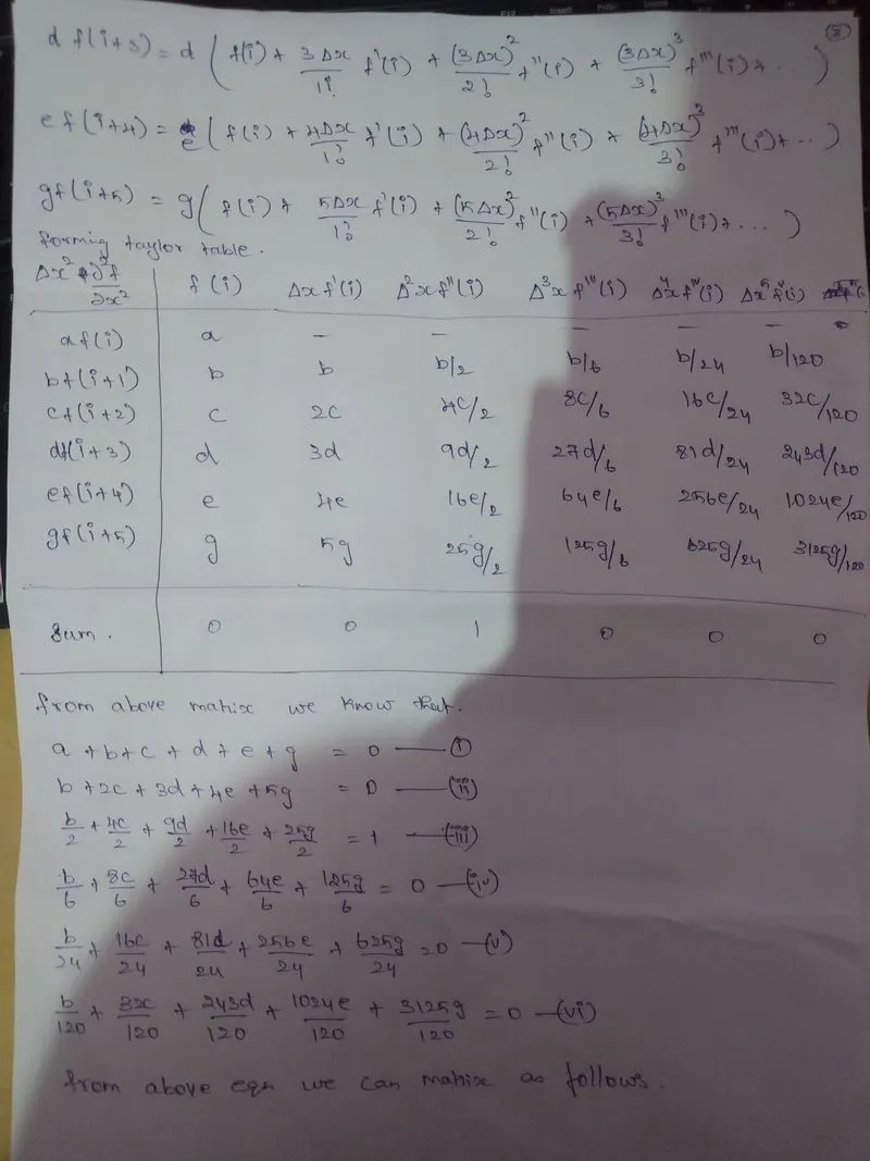
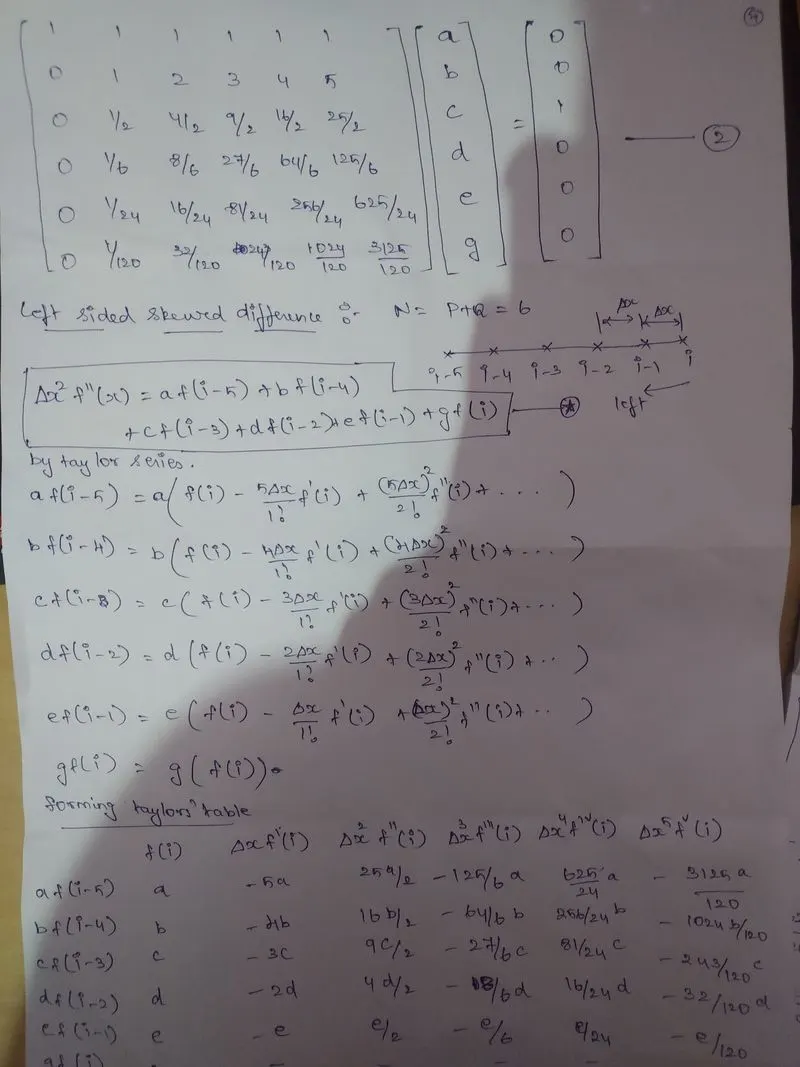
to derive the following 4th order approximations of the second-order derivative.
1. Central difference
2. Skewed right-sided difference
3. Skewed left-sided difference.
given:
After deriving these schemes, prove that your skewed schemes are fourth-order accurate i.e the thumb rule given in HINT (ii).
Once you have done this, write a program in Matlab to evaluate the second-order derivative of the analytical function exp(x)*cos(x) and compare it with the 3 numerical approximations that you have derived.
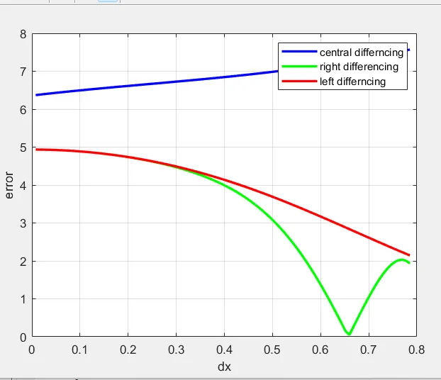
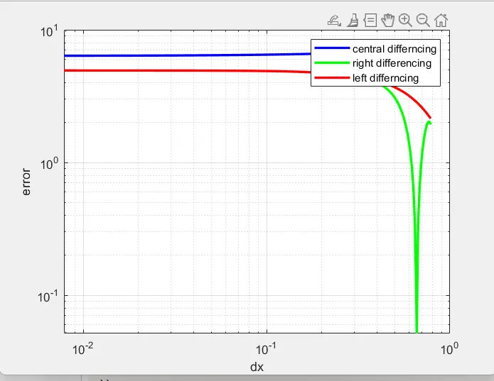
Provide a plot that compares the absolute error between the above-mentioned schemes
In your own words, describe why a skewed scheme is useful? What can a skewed scheme do that a CD scheme cannot?
HINT :
i) The order of accuracy P = Number of nodes in the stencil N - order of derivative Q + 1 for symmetric/central schemes
ii) The order of accuracy P = Number of nodes in the stencil N - order of derivative Q for one-sided/skewed schemes
iii) Solve the system of equations using the matrix inversion method in Matlab to obtain the taylor table coefficients and use them directly in the numerical approximation statements to avoid input errors.
Taylor's Series:
A Taylor Series is an expansion of some function into an infinite sum of terms, where each term has a larger exponent like x, x2, x3, etc.
Example: The taylor series for the function ex��:
ex = 1+x+ x22! + x33! + x44! + x55! +...
says that the function:ex is equal to the infinite sum of terms:1 + x + x2/2! + x3/3! + ... etc.
derivation:
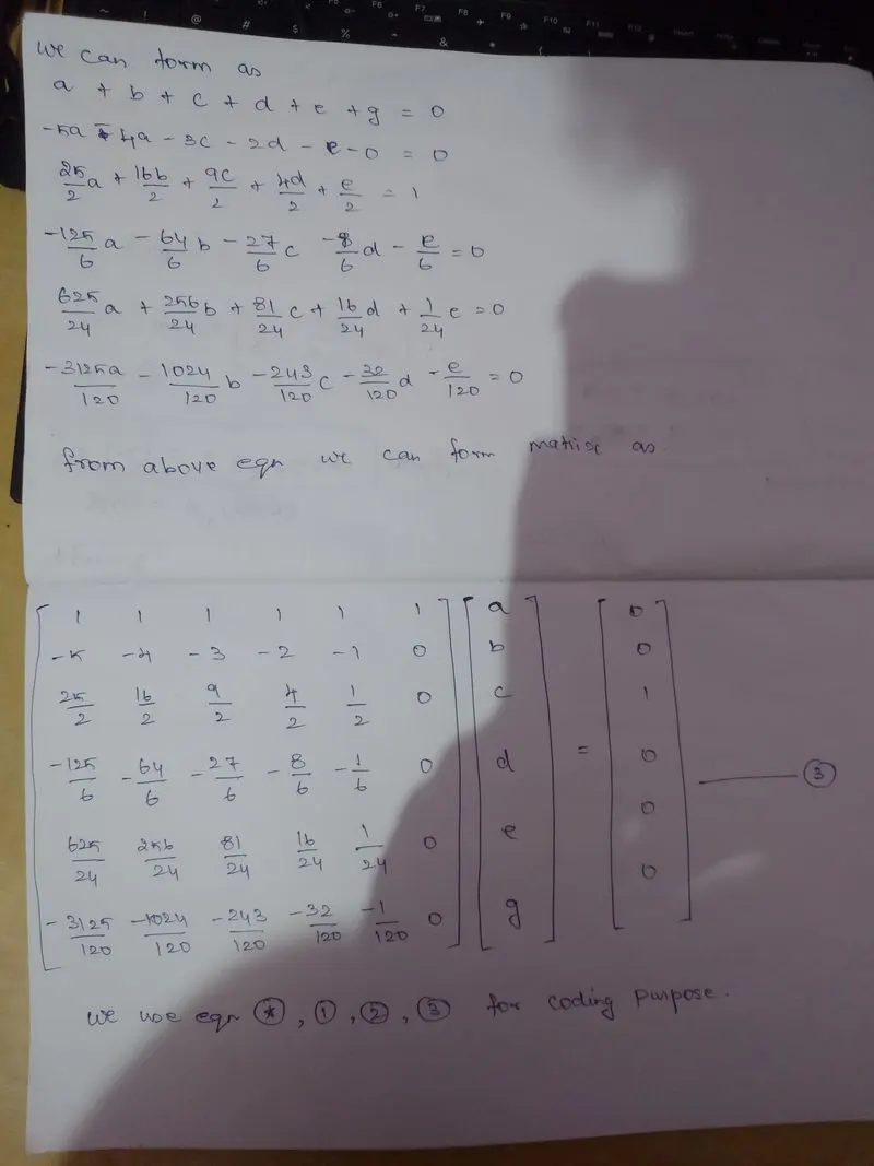
Coding:
lets take or assume f(x) = exp(x) * cos(x)
also f''(x)=-2 exp(x) * sin(x)........analytical derivative function equation
clear all
close all
clc

%f(x) = exp. (x) * cos(x)
%f''(x) = -2 exp(x)*sin(x)

x = pi/3;
dx = linspace(pi/4,pi/400,100);

% calculating analytical value of second order function
analytical_derivative = -2*exp(x)*sin(x);

%central differencing scheme
a_central = [1 1 1 1 1;-2 -1 0 1 2;2 1/2 0 1/2 2;-4/3 -1/6 0 1/6 4/3;2/3 1/24 0 1/24 2/3];
b_central = [0;0;1;0;0]
c_central = inv(a_central)*b_central;

% c_central(1)*(exp(x-(dx)*2).*cos(x-(dx)*2))

%calculative second order derivative
central_differencing = (c_central(1)*(exp(x-(dx)*2).*cos(x-(dx)*2)))+(c_central(2)*(exp(x-(dx)).*cos(x-(dx))))+(c_central(1)*(exp(x).*cos(x)))+(c_central(1)*(exp(x+(dx)).*cos(x+(dx))))+(c_central(1)*(exp(x+(dx)*2).*cos(x+(dx)*2)))

% error
error_central = abs(analytical_derivative-central_differencing)

% skewed right sided differnce

a_right = [1 1 1 1 1 1;0 1 2 3 4 5;0 1/2 4/2 9/2 16/2 25/2;0 1/6 8/6 27/6 64/6 125/6;0 1/24 16/24 81/24 256/24 625/24;0 1/120 32/120 243/120 1024/120 3125/120];

b_right = [0;0;1;0;0;0]

c_right = inv(a_right)*b_right;

%calaculating right sided skewed difference c_right(1)*(exp(x-(dx)*2).*cos(x-(dx)*2))

right_differencing = (c_right(1)*(exp(x).*cos(x)))+(c_right(2)*(exp(x+(dx)).*cos(x+(dx))))+(c_right(3)*(exp(x+(dx)*2).*cos(x+(dx)*2)))+(c_right(4)*(exp(x+(dx)*3).*cos(x+(dx)*3)))+(c_right(5)*(exp(x+(dx)*4).*cos(x+(dx)*4)))+(c_right(6)*(exp(x+(dx)*5).*cos(x+(dx)*5)))

% error

error_right = abs(analytical_derivative-right_differencing)

% skewed left sided difference

a_left = [1 1 1 1 1 1;-5 -4 -3 -2 -1 0;25/2 16/2 9/2 4/2 1/2 0;-125/6 -64/6 -27/6 -8/6 -1/6 0;625/24 256/24 81/24 16/24 1/24 0;-3125/120 -1024/120 -243/120 -32/120 -1/120 0]
b_left = [0;0;1;0;0;0]

c_left = inv(a_left)*b_left;

%calculating left sided differnce  c_left(1)*(exp(x).*cos(x))

left_differncing = (c_left(1)*(exp(x-(dx)*5).*cos(x-(dx)*5)))+(c_left(2)*(exp(x-(dx)*4).*cos(x-(dx)*4)))+(c_left(3)*(exp(x-(dx)*3).*cos(x-(dx)*3)))+(c_left(4)*(exp(x-(dx)*2).*cos(x-(dx)*2)))+(c_left(5)*(exp(x-(dx)).*cos(x-(dx))))+(c_left(6)*(exp(x).*cos(x)));

%error
 error_left = abs(analytical_derivative-left_differncing);

 % plotting

figure(1)
plot(dx,error_central,'b','LineWidth',2)
hold on
grid on
plot(dx,error_right,'g','LineWidth',2)
hold on
plot(dx,error_left,'r','LineWidth',2)
xlabel("dx")
ylabel("error")
legend("central differncing","right differencing","left differncing");

figure(2)
loglog(dx,error_central,'b','LineWidth',2)
hold on
grid on
loglog(dx,error_right,'g','LineWidth',2)
hold on
loglog(dx,error_left,'r','LineWidth',2)
xlabel("dx")
ylabel("error")
legend("central differncing","right differencing","left differncing");
OUTPUT :
central_differencing =

  Columns 1 through 7

    2.6359    2.6151    2.5946    2.5743    2.5543    2.5346    2.5152

  Columns 8 through 14

    2.4960    2.4771    2.4585    2.4402    2.4222    2.4044    2.3869

  Columns 15 through 21

    2.3696    2.3527    2.3360    2.3195    2.3033    2.2874    2.2718

  Columns 22 through 28

    2.2563    2.2412    2.2262    2.2116    2.1971    2.1829    2.1689

  Columns 29 through 35

    2.1552    2.1417    2.1284    2.1153    2.1024    2.0897    2.0772

  Columns 36 through 42

    2.0650    2.0529    2.0410    2.0293    2.0177    2.0063    1.9951

  Columns 43 through 49

    1.9841    1.9732    1.9625    1.9519    1.9415    1.9312    1.9210

  Columns 50 through 56

    1.9109    1.9010    1.8912    1.8814    1.8718    1.8623    1.8529

  Columns 57 through 63

    1.8435    1.8342    1.8250    1.8159    1.8068    1.7978    1.7888

  Columns 64 through 70

    1.7799    1.7710    1.7621    1.7533    1.7445    1.7357    1.7269

  Columns 71 through 77

    1.7181    1.7093    1.7004    1.6916    1.6827    1.6738    1.6649

  Columns 78 through 84

    1.6560    1.6469    1.6379    1.6287    1.6195    1.6103    1.6009

  Columns 85 through 91

    1.5915    1.5820    1.5724    1.5627    1.5529    1.5429    1.5329

  Columns 92 through 98

    1.5227    1.5124    1.5020    1.4915    1.4807    1.4699    1.4589

  Columns 99 through 100

    1.4477    1.4363


error_central =

  Columns 1 through 7

    7.5717    7.5509    7.5303    7.5101    7.4901    7.4704    7.4509

  Columns 8 through 14

    7.4318    7.4129    7.3943    7.3760    7.3579    7.3401    7.3226

  Columns 15 through 21

    7.3054    7.2884    7.2717    7.2553    7.2391    7.2232    7.2075

  Columns 22 through 28

    7.1921    7.1769    7.1620    7.1473    7.1329    7.1187    7.1047

  Columns 29 through 35

    7.0909    7.0774    7.0641    7.0510    7.0381    7.0255    7.0130

  Columns 36 through 42

    7.0007    6.9886    6.9767    6.9650    6.9535    6.9421    6.9309

  Columns 43 through 49

    6.9199    6.9090    6.8982    6.8877    6.8772    6.8669    6.8567

  Columns 50 through 56

    6.8467    6.8367    6.8269    6.8172    6.8076    6.7980    6.7886

  Columns 57 through 63

    6.7793    6.7700    6.7608    6.7517    6.7426    6.7336    6.7246

  Columns 64 through 70

    6.7157    6.7068    6.6979    6.6891    6.6802    6.6714    6.6626

  Columns 71 through 77

    6.6538    6.6450    6.6362    6.6273    6.6185    6.6096    6.6007

  Columns 78 through 84

    6.5917    6.5827    6.5736    6.5645    6.5553    6.5460    6.5367

  Columns 85 through 91

    6.5273    6.5177    6.5081    6.4984    6.4886    6.4787    6.4686

  Columns 92 through 98

    6.4585    6.4482    6.4378    6.4272    6.4165    6.4056    6.3946

  Columns 99 through 100

    6.3834    6.3721


b_right =

     0
     0
     1
     0
     0
     0


right_differencing =

  Columns 1 through 7

   -6.8689   -6.9403   -6.9668   -6.9540   -6.9068   -6.8300   -6.7277

  Columns 8 through 14

   -6.6038   -6.4618   -6.3047   -6.1354   -5.9564   -5.7700   -5.5782

  Columns 15 through 21

   -5.3827   -5.1853   -4.9872   -4.7897   -4.5937   -4.4004   -4.2103

  Columns 22 through 28

   -4.0241   -3.8424   -3.6657   -3.4942   -3.3283   -3.1680   -3.0137

  Columns 29 through 35

   -2.8653   -2.7228   -2.5864   -2.4558   -2.3311   -2.2121   -2.0987

  Columns 36 through 42

   -1.9907   -1.8880   -1.7903   -1.6976   -1.6096   -1.5261   -1.4469

  Columns 43 through 49

   -1.3718   -1.3006   -1.2332   -1.1692   -1.1086   -1.0511   -0.9966

  Columns 50 through 56

   -0.9449   -0.8958   -0.8492   -0.8049   -0.7628   -0.7227   -0.6846

  Columns 57 through 63

   -0.6482   -0.6135   -0.5805   -0.5489   -0.5187   -0.4899   -0.4622

  Columns 64 through 70

   -0.4358   -0.4105   -0.3862   -0.3629   -0.3406   -0.3191   -0.2986

  Columns 71 through 77

   -0.2789   -0.2599   -0.2418   -0.2244   -0.2077   -0.1918   -0.1765

  Columns 78 through 84

   -0.1619   -0.1480   -0.1348   -0.1221   -0.1102   -0.0988   -0.0881

  Columns 85 through 91

   -0.0780   -0.0686   -0.0597   -0.0515   -0.0439   -0.0368   -0.0305

  Columns 92 through 98

   -0.0247   -0.0195   -0.0149   -0.0110   -0.0076   -0.0049   -0.0027

  Columns 99 through 100

   -0.0012   -0.0003


error_right =

  Columns 1 through 7

    1.9332    2.0046    2.0311    2.0182    1.9711    1.8943    1.7920

  Columns 8 through 14

    1.6681    1.5260    1.3690    1.1996    1.0207    0.8342    0.6424

  Columns 15 through 21

    0.4470    0.2495    0.0514    0.1461    0.3420    0.5354    0.7255

  Columns 22 through 28

    0.9116    1.0933    1.2701    1.4415    1.6075    1.7677    1.9221

  Columns 29 through 35

    2.0705    2.2129    2.3494    2.4799    2.6047    2.7237    2.8371

  Columns 36 through 42

    2.9451    3.0478    3.1454    3.2381    3.3261    3.4096    3.4888

  Columns 43 through 49

    3.5639    3.6351    3.7026    3.7665    3.8271    3.8846    3.9391

  Columns 50 through 56

    3.9908    4.0399    4.0866    4.1309    4.1730    4.2130    4.2512

  Columns 57 through 63

    4.2875    4.3222    4.3553    4.3869    4.4170    4.4459    4.4735

  Columns 64 through 70

    4.4999    4.5253    4.5496    4.5728    4.5952    4.6166    4.6372

  Columns 71 through 77

    4.6569    4.6758    4.6939    4.7113    4.7280    4.7440    4.7592

  Columns 78 through 84

    4.7738    4.7877    4.8010    4.8136    4.8256    4.8369    4.8476

  Columns 85 through 91

    4.8577    4.8672    4.8760    4.8843    4.8919    4.8989    4.9053

  Columns 92 through 98

    4.9111    4.9163    4.9208    4.9248    4.9281    4.9309    4.9330

  Columns 99 through 100

    4.9345    4.9354


a_left =

    1.0000    1.0000    1.0000    1.0000    1.0000    1.0000
   -5.0000   -4.0000   -3.0000   -2.0000   -1.0000         0
   12.5000    8.0000    4.5000    2.0000    0.5000         0
  -20.8333  -10.6667   -4.5000   -1.3333   -0.1667         0
   26.0417   10.6667    3.3750    0.6667    0.0417         0
  -26.0417   -8.5333   -2.0250   -0.2667   -0.0083         0


b_left =

     0
     0
     1
     0
     0
     0

>>
>>
Plot will be
OBSERVATION:
- It has been concluded that the errors in central differencing method is much less than the other two schemes.
- The left-sided skewed and right sided skewed schemes shows nearly same amount of errors.
Why Skewed scheme is useful?
The skewed scheme is useful because it is necessary to compute the grids at the corners also which central differecing scheme is unable to do. Symmetric nodes does not present on the corners so that CD can not be implemented in such conditions.