Week 3.5 - Deriving 4th order approximation of a 2nd order derivative using Taylor Table method

AIM

Derive the following 4th order approximations of the second-order derivative.

1. Central difference

2. Skewed right-sided difference

3. Skewed left-sided difference

After deriving these schemes, prove that your skewed schemes are fourth-order accurate i.e the thumb rule given in HINT (ii).

Once you have done this, write a program in Matlab to evaluate the second-order derivative of the analytical function exp(x)*cos(x) and compare it with the 3 numerical approximations that you have derived.

Provide a plot that compares the absolute error between the above-mentioned schemes

In your own words, describe why a skewed scheme is useful? What can a skewed scheme do that a CD scheme cannot?

OBJECTIVE-1 →Deriving the central, skewed right-sided and skewed left-sided differencing schemes.

1. 4th order Approximations of 2nd order Derivaive using CENTRAL DIFFERENCING

Number of nodes in CD = p + q - 1

where, p→ order of derivative, q → order of approximation

∴ Number of nodes in CD = 2 + 4 - 1 = 5, (i.e. (i−2),(i−1),(i),(i+1),(i+2)) →

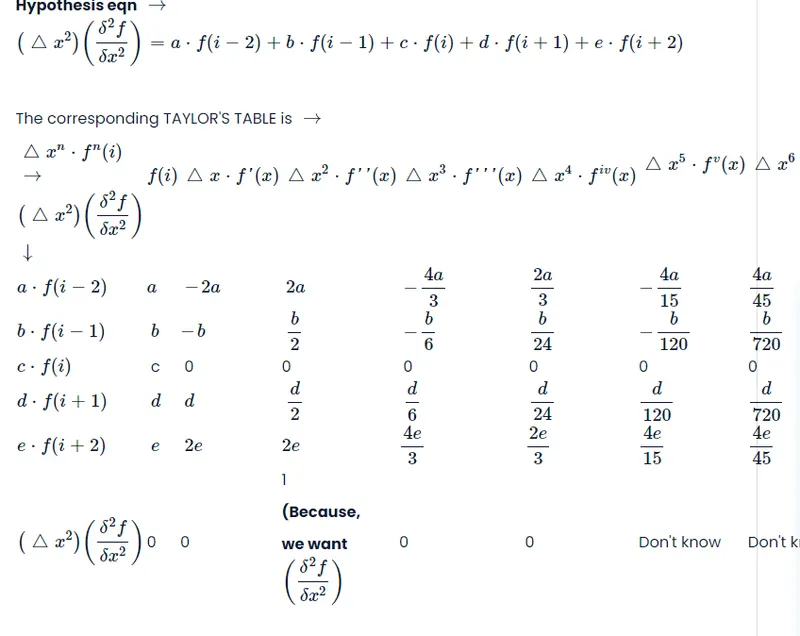
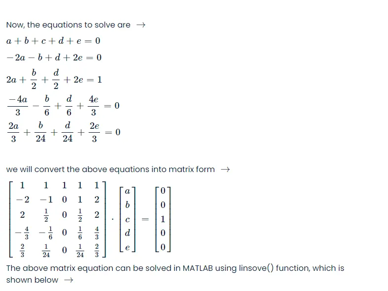
% PROGRAM TO SOLVE THE MATRIX EQUATION FORMED FOR CALCULATING THE CENTRAL
% DIFFERENCING SCHEME

close all
clear all
clc

A = [1 1 1 1 1;-2 -1 0 1 2;2 1/2 0 1/2 2;-4/3 -1/6 0 1/6 4/3;2/3 1/24 0 1/24 2/3]
B = [0;0;1;0;0]
X = linsolve(A,B)

Output →→

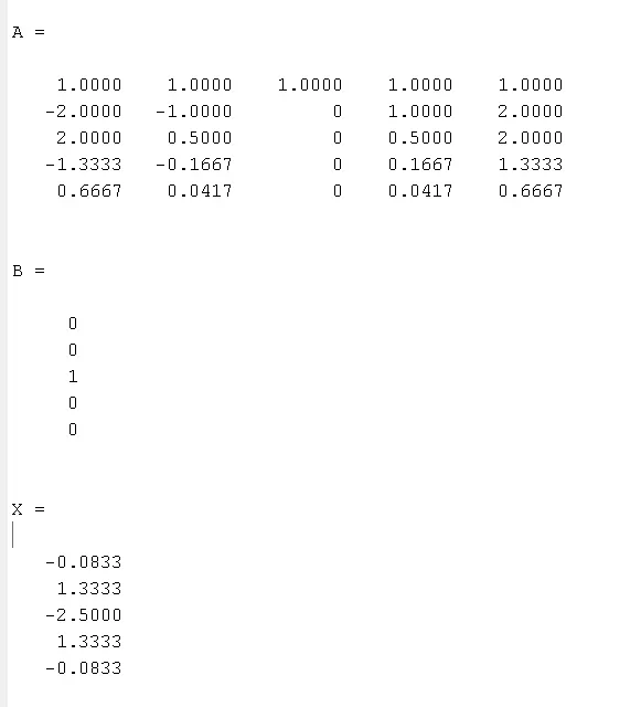
You can see the X value in the above image is for a=−0.0833,b=1.3333,c=−2.5,d=1.3333,e=−0.0833]And it is clear that the the values of a=e and b=d

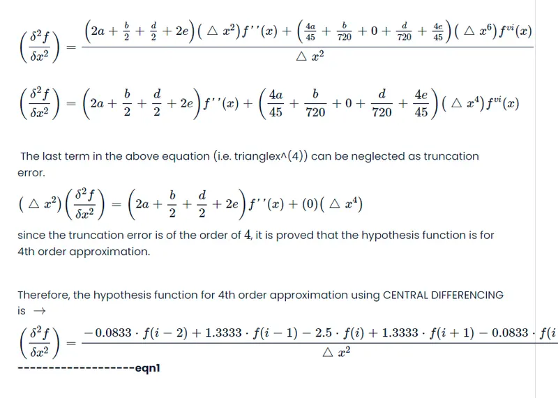
Proof of Hypothesis function having a truncation error of order 4 →

2. 4th order Approximations of 2nd order Derivaive using SKEWED RIGHT-SIDED DIFFERENCING SCHEME

Number of nodes in CD = p + q

where, p→order of derivative, q → order of approximation

∴ Number of nodes in CD = 2 + 4 = 6, (i.e. (i),(i+1),(i+2),(i+3),(i+4),(i+5)

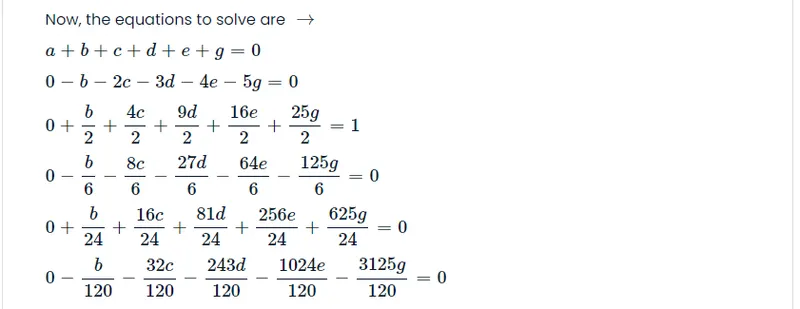
Hypothesis eqn →

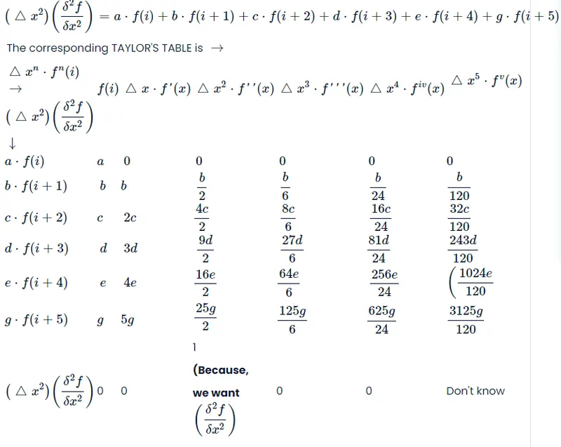
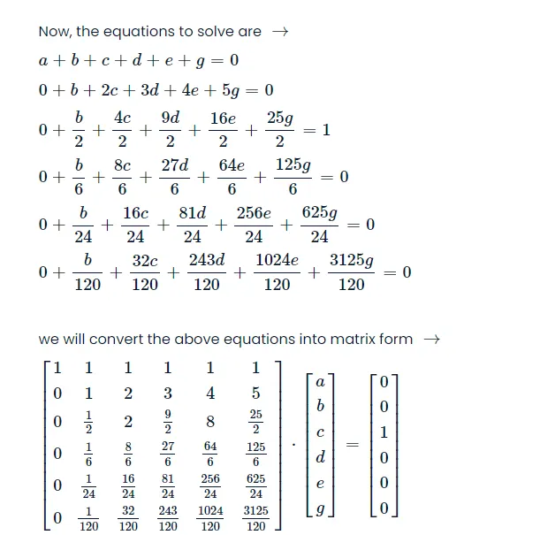
The above matrix equation can be solved in MATLAB using linsove() function, which is shown below →

% PROGRAM TO SOLVE THE MATRIX EQUATION FORMED FOR CALCULATING THE SKEWED RIGHT-SIDED SCHEME

close all
clear all
clc

A = [1 1 1 1 1 1;
     0 1 2 3 4 5;
     0 1/2 2 9/2 8 25/2;
     0 1/6 8/6 27/6 64/6 125/6;
     0 1/24 16/24 81/24 256/24 625/24;
     0 1/120 32/120 243/120 1024/120 3125/120]
B = [0;0;1;0;0;0]
X = linsolve(A,B)

Output →→

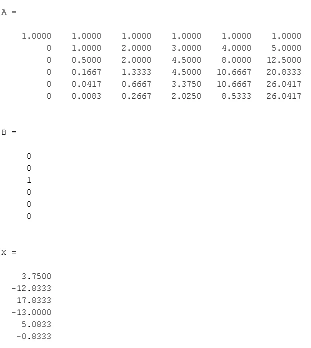
You can see the X value in the above image is for

a=3.75,b=−12.8333,c=17.8333,d=−13,e=5.0833,g=−0.8333.

Therefore, the hypothesis function for 4th order approximation using SKEWED RIGHT-SIDED DIFFERENCING is →

3. 4th order Approximations of 2nd order Derivaive using SKEWED LEFT-SIDED DIFFERENCING SCHEME

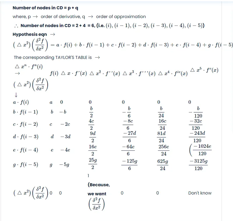
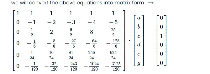
The above matrix equation can be solved in MATLAB using linsove() function, which is shown below →

% PROGRAM TO SOLVE THE MATRIX EQUATION FORMED FOR CALCULATING THE LEFT-SIDED DIFFERENCING SCHEME

close all
clear all
clc

% A = [1 1 1 1 1;-2 -1 0 1 2;2 1/2 0 1/2 2;-4/3 -1/6 0 1/6 4/3;2/3 1/24 0 1/24 2/3]
% B = [0;0;1;0;0]
% X = linsolve(A,B)

A = [1 1 1 1 1 1;
     0 -1 -2 -3 -4 -5;
     0 1/2 2 9/2 8 25/2;
     0 -1/6 -8/6 -27/6 -64/6 -125/6;
     0 1/24 16/24 81/24 256/24 625/24;
     0 -1/120 -32/120 -243/120 -1024/120 -3125/120]
B = [0;0;1;0;0;0]
X = linsolve(A,B)

Output →→

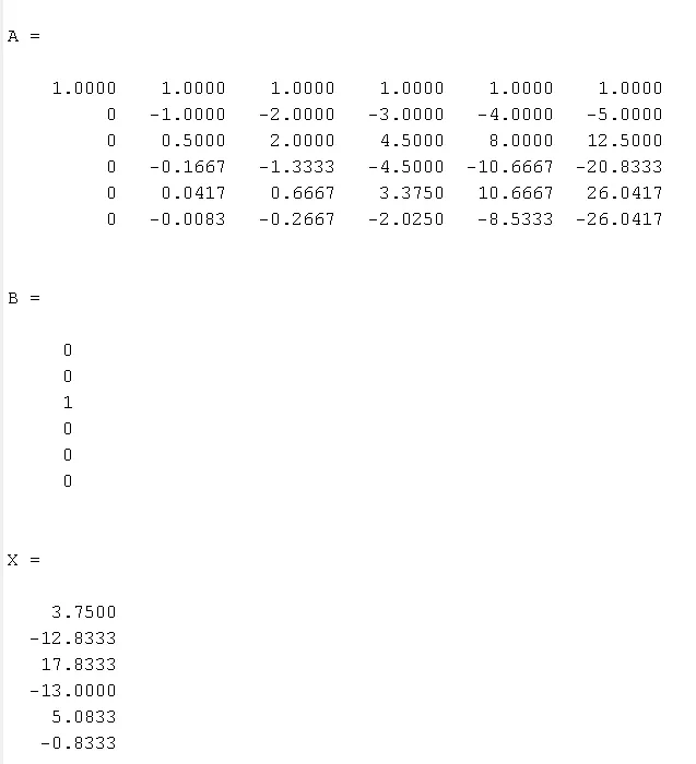
You can see the X value in the above image is for

a=3.75,b=−12.8333,c=17.8333,d=−13,e=5.0833,g=−0.8333.

It is same as that of the skewed right handed differencing scheme.

Therefore, the hypothesis function for 4th order approximation using SKEWED RIGHT-SIDED DIFFERENCING is →→

(δ2fδx2)=3.75⋅f(i)−12.8333⋅f(i−1)+17.8333⋅f(i−2)−13⋅f(i−3)+5.0833⋅f(i−4)−0.8333⋅f(i−5)/△x2..........................................................eqn3

OBJECTIVE-2 →write a program in Matlab to evaluate the second-order derivative of the analytical function exp(x)*cos(x) and compare it with the 3 numerical approximations that you have derived. Provide a plot that compares the absolute error between the above-mentioned schemes

% Program to evaluate the second order derivative for 'exp(x)*cos(x)',
% using skewed left-sided, central and skewed right-sided differencing
% scheme

close all                                                        %closes all the matlab windows, plots etc
clear all                                                        %clears all the workspace variables
clc                                                              %clears the command window

% ANALYTICAL FUNCTION, f(x)=exp(x)*cos(x)


%ANALYTICAL DERIVATIVE
%f''(x) = -2*exp(x)*sin(x)
x =pi/3;                                                             %grid point at which the derivative has to be found
analytical_second_derivative = -2*exp(x)*sin(x)                      % analytical derivative of function


%NUMERICAL DERIVATIVE

dx=linspace(pi/4000,pi/40,20);                                       % grid spacing in 3d

for i=1:20
    %SECOND order approximation
    %skewed left-sided differencing[S-LS-D ] [f''(x)]
    %f''(x) =(3.75*f(i)-12.8333*f(i-1)+17.8333*f(i-2)-13*f(i-3)+5.0833*f(i-4)-0.8333*f(i-5)/(dx^2)
    skewed_left_sided_differencing(i) = (3.75*(exp(x)*cos(x)) - 12.8333*(exp(x-dx(i))*cos(x-dx(i))) + 17.8333*(exp(x-2*dx(i))*cos(x-2*dx(i))) - 13*(exp(x-3*dx(i))*cos(x-3*dx(i))) + 5.0833*(exp(x-4*dx(i))*cos(x-4*dx(i))) - 0.8333*(exp(x-5*dx(i))*cos(x-5*dx(i))))/(dx(i)^2);       %skewed left-sided differencing for 2nd order derivative


    %SECOND order approximation
    %central differencing of second derivative[C-D] [f''(x)]
    %f''(x)=(-0.0833*f(i-2) + 1.3333*f(i-1) - 2.5*f(i) + 1.3333*f(i+1) - 0.0833*f(i+2))/(dx^2)
    central_differencing_second_order(i) = (-0.0833*(exp(x-2*dx(i))*cos(x-2*dx(i))) + 1.3333*(exp(x-dx(i))*cos(x-dx(i))) - 2.5*(exp(x)*cos(x)) + 1.3333*((exp(x+dx(i))*cos(x+dx(i)))) - 0.0833*(exp(x+2*dx(i))*cos(x+2*dx(i))))/(dx(i)^2);                                             %central differencing for 2nd order derivative


    %SECOND order approximation
    %skewed right-sided differencing [S-RS-D] [f''(x)]
    %f''(x) = (3.75*f(i)-12.8333*f(i+1)+17.8333*f(i+2)-13*f(i+3)+5.0833*f(i+4)-0.8333*f(i+5)/(dx^2)
    skewed_right_sided_differencing(i) = (3.75*(exp(x)*cos(x)) - 12.8333*(exp(x+dx(i))*cos(x+dx(i))) + 17.8333*(exp(x+2*dx(i))*cos(x+2*dx(i))) - 13*(exp(x+3*dx(i))*cos(x+3*dx(i))) + 5.0833*(exp(x+4*dx(i))*cos(x+4*dx(i))) - 0.8333*(exp(x+5*dx(i))*cos(x+5*dx(i))))/(dx(i)^2);      %skewed right-sided differencing for 2nd order derivative 
                                                           

    %ERROR calculation
    left_skewed_error(i) = abs(skewed_left_sided_differencing(i) - analytical_second_derivative);                   %error calculation between S-LS-D & analytical derivative
    central_differencing_error(i) = abs(central_differencing_second_order(i) - analytical_second_derivative);       %error calculation between C-D & analytical derivative
    right_skewed_error(i) = abs(skewed_right_sided_differencing(i) - analytical_second_derivative);                 %error calculation between S-RS-D & analytical derivative

end

display(left_skewed_error)
display(central_differencing_error)
display(right_skewed_error)
% display(dx)

figure(1)       
loglog(dx,left_skewed_error,'-',dx,central_differencing_error,':',dx,right_skewed_error,'-.','color','r')
xlabel('log dx')
ylabel('log Error')
title("Error for numerical Approximation for dx value for 20 number's ranging from pi/4000 to pi/40 ")
legend("left skewed scheme","central differencing scheme","right skewed scheme")

%Slope of the curve obtained

slope_of_left_skewed_scheme = mean(diff(left_skewed_error)./diff(dx))
slope_of_central_differencing_scheme = mean(diff(central_differencing_error)./diff(dx))
slope_of_right_skewed_scheme = mean(diff(right_skewed_error)./diff(dx))

output→→

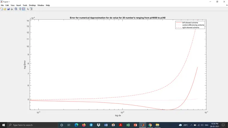
COMPARISON →

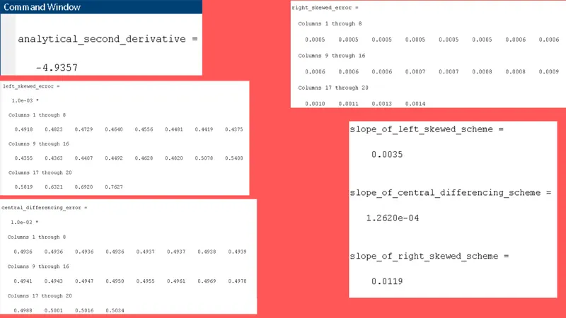
• you can see in the above plots, the error is more for skewed schemes than for the central differencing schemes.
• the errors, skewed left sided has started from 4.92⋅10−44.92⋅10-4, for central differencing - 4.935⋅10−44.935⋅10-4 and for the right sided scheme- 4.955⋅10−44.955⋅10-4. By the end of the curves, the error for central differencing is low and mostly linear, as comared to the skewed schems.
• the large error values for skewed schemes than for the central differencing is because the no: of nodes is only 2-points apart, whereas in the skewed schemes, it is 5-points apart.
• as the dx value reaches 1 or exceeds 1, then the error values will become unstable and the variations will much more.
• also, the slope values of CD is less than the skewed schems. It means as the dx progresses, the frequency of error formation across the y-axis is constant. hence we get a linear plot and a minimum slope value.

OBJECTIVE-3 → Describe why a skewed scheme is useful? What can a skewed scheme do that a CD scheme cannot?

suppose we have to find the heat transfer values at the end of a concrete wall. In that case we are restricted with grid points only to one side, i.e. either left or right. In that scenarios, we cannot go for central differencing, since symmetric nodes is not possible.