Week 3.5 - Deriving 4th order approximation of a 2nd order derivative using Taylor Table method

AIM

To derive the 4th order approximations of the second-order derivative using Central difference, Skewed right-sided difference, Skewed left-sided difference schemes and prove that our skewed schemes are fourth-order accurate. Also to write a program in Matlab to evaluate the second-order derivative of the analytical function exp(x)*cos(x) and compare it with the 3 numerical approximations that have been derived.

DERIVATION

Using Taylor Table method one can easily derive an equation for any order of accuracy and prove that the skewed schemes are fourth-order accurate using the following relation -

i) The order of accuracy P = Number of nodes in the stencil N - order of derivative Q + 1 for symmetric/central schemes

ii) The order of accuracy P = Number of nodes in the stencil N - order of derivative Q for one-sided/skewed schemes

fourth_order_approx_central = ((-0.0833*f(i-2)) + (1.333*f(i-1)) + (-2.5*f(i)) + (1.333*f(i+1)) + (-0.0833*f(i+2))) / (dx^2)

fourth_order_approx_rskewed = ((3.7500*f(i)) + (-12.8333*f(i+1)) + (17.8333*f(i+2)) + (-13.0000*f(i+3)) + ( 5.0833*f(i+4)) + (-0.8333*f(i+5))) / (dx^2)

fourth_order_approx_lskewed = ((-0.8333*f(i-5)) + (5.0833*f(i-4)) + (-13*f(i-3)) + (17.8333*f(i-2)) + (-12.8333*f(i-1)) + (3.7500*f(i)) / (dx^2)

Proof -

Number of nodes in the stencil N = 6; order of derivative Q = 2;

Therefore the order of accuracy P = 6 - 2 = 4.

PROGRAM

close all
clear
clc

%% Inputs to the given problem
x = pi/3;
dx = pi/30;

%% Analytical solution for the 2nd order derivative of the given function exp(x)*cos(x)

exact_sol = -2*exp(x)*sin(x)

%% Fourth order approximation of 2nd order derivative using central difference scheme
e = exp(x - (2*dx))*cos(x - (2*dx));
d = exp(x - dx)*cos(x - dx);
c = exp(x)*cos(x);
b = exp(x + dx)*cos(x + dx);
a = exp(x + (2*dx))*cos(x + (2*dx));

fourth_order_approx_central = ((-0.0833*e) + (1.333*d) + (-2.5*c) + (1.333*b) + (-0.0833*a)) / (dx^2)

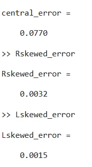
central_error = abs(fourth_order_approx_central - exact_sol)

%% Fourth order approximation of 2nd order derivative using right skewed scheme 

q2 = [1 1 1 1 1 1; 0 1 2 3 4 5; 0 1/2 2 9/2 8 25/2; 0 1/6 4/3 9/2 32/3 125/6; 0 1/24 2/3 27/8 64/6 625/24; 0 1/120 8/30 243/120 1024/120 3125/120];
w2 = [0; 0; 1; 0; 0; 0];
e2 = q2\w2;

a1 = exp(x)*cos(x);
b1 = exp(x + dx)*cos(x + dx);
c1 = exp(x + 2*dx)*cos(x + 2*dx);
d1 = exp(x + 3*dx)*cos(x + 3*dx);
e1 = exp(x + 4*dx)*cos(x + 4*dx);
f1 = exp(x + 5*dx)*cos(x + 5*dx);

fourth_order_approx_rskewed = ((3.7500*a1) + (-12.8333*b1) + (17.8333*c1) + (-13.0000*d1) + ( 5.0833*e1) + (-0.8333*f1)) / (dx^2)

Rskewed_error = abs(fourth_order_approx_rskewed - exact_sol)

%% Fourth order approximation of 2nd order derivative using left skewed scheme
q3 = [1 1 1 1 1 1; -5 -4 -3 -2 -1 0; 25/2 8 9/2 2 0.5 0; -125/6 -64/6 -27/6 -8/6 -1/6 0; 625/24 256/24 81/24 16/24 1/24 0; -3125/120 -1024/120 -243/120 -32/120 -1/120 0];
w3 = [0; 0; 1; 0; 0; 0];
e3 = q3\w3;

f2 = exp(x)*cos(x);
e2 = exp(x - dx)*cos(x - dx);
d2 = exp(x - 2*dx)*cos(x - 2*dx);
c2 = exp(x - 3*dx)*cos(x - 3*dx);
b2 = exp(x - 4*dx)*cos(x - 4*dx);
a2 = exp(x - 5*dx)*cos(x - 5*dx);

fourth_order_approx_lskewed = ((-0.8333*a2) + (5.0833*b2) + (-13*c2) + (17.8333*d2) + (-12.8333*e2) + (3.7500*f2)) / (dx^2)

Lskewed_error = abs(exact_sol - fourth_order_approx_lskewed)

%% Plotting

bar(central_error)
hold on
bar(Rskewed_error)
hold on
bar(Lskewed_error)
legend('central_error', 'Rskewed_error', 'Lskewed_error')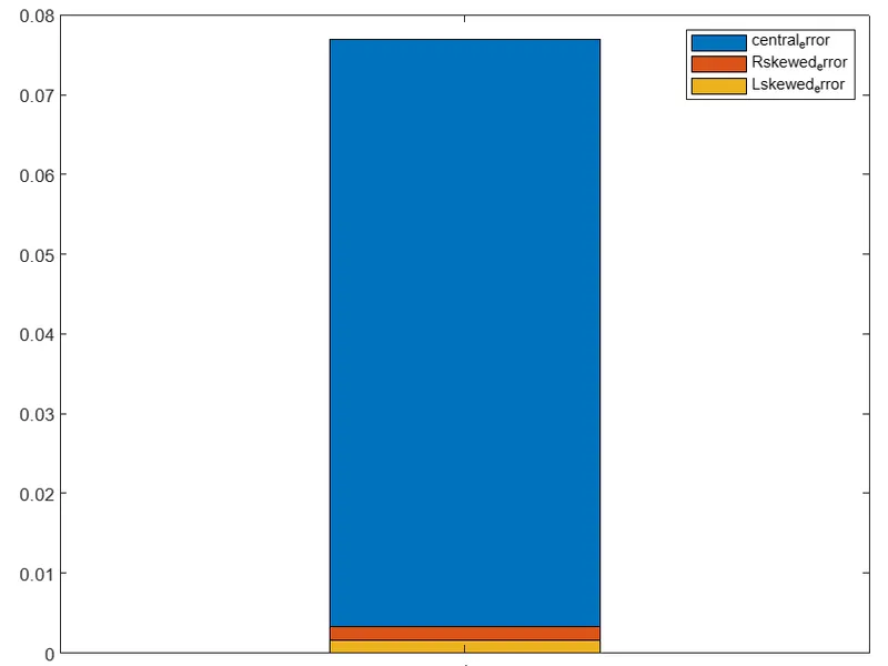

From the above bar plot it is clearly visible that the error is reduced when a skewed scheme is used to fourth order approximation by a factor of 1.

OUTPUT