Week 3.5 - Deriving 4th order approximation of a 2nd order derivative using Taylor Table method

Aim

Derive the following 4th order approximations of the second-order derivative.

1. Central difference

2. Skewed right-sided difference

3. Skewed left-sided difference

After deriving these schemes, prove that your skewed schemes are fourth-order accurate.

Once you have done this, write a program in Matlab to evaluate the second-order derivative of the analytical function exp(x)*cos(x) and compare it with the 3 numerical approximations that you have derived.

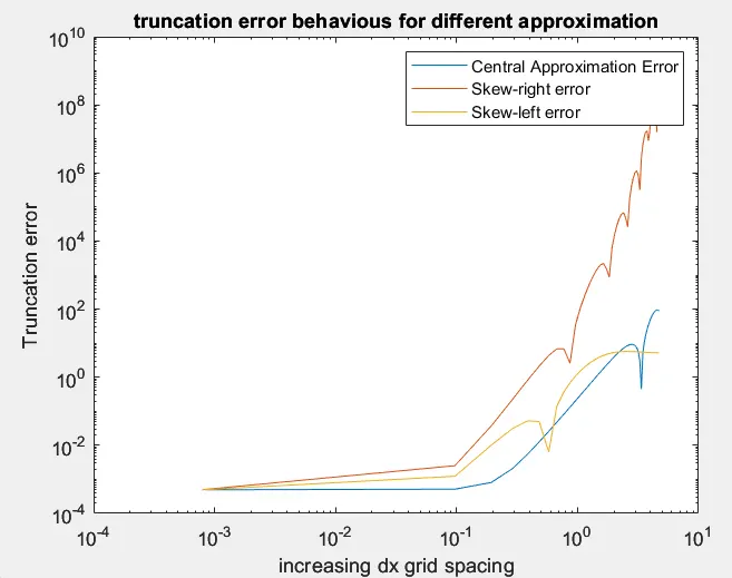
Provide a plot that compares the absolute error between the above-mentioned schemes.

Theory

Taylor series is the polynomial or a function of an infinite sum of terms. Each successive term will have a larger exponent or higher degree than the preceding term.

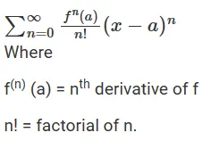
Assume that if f(x) be a real or composite function, which is a differentiable function of a neighbourhood number that is also real or composite. Then, the Taylor series describes the following power series :

In terms of sigma notation, the Taylor series can be written as

Proof

We know that the power series can be defined as

When x = 0,

f(x)= a₀

So, differentiate the given function, it becomes,

f’(x) = a₁+ 2a₂x + 3a₃x² + 4a₄x³ +….

Again, when you substitute x = 0, we get

f’(0) =a₁

So, differentiate it again, we get

f”(x) = 2a₂ + 6a₃x +12a₄x² + …

Now, substitute x=0 in second-order differentiation, we get

f”(0) = 2a₂

Therefore, [f”(0)/2!] = a₂

By generalising the equation, we get

f ⁿ (0) / n! = a_n

Now substitute the values in the power series we get,

Generalise f in more general form, it becomes

f(x) = b + b₁ (x-a) + b₂( x-a)² + b₃ (x-a)³+ ….

Now, x = a, we get

b_n = fⁿ(a) / n!

Now, substitute b_n in a generalised form

Hence, the Taylor series is proved.

For example, the below graph shows approximation at x=0, here we can see that as the number of terms increases the two curves becomes coincident.

The exponential function ex (in blue), and the sum of the first n + 1 terms of its Taylor series at 0 (in red).

Deriving the given 4th order approximations of the second-order derivative by following methods

1. Central difference

The number of Nodes required for 4th order approximation of a second-order derivative can be given by the equation

N=P+Q−1N=P+Q-1 where

NN is the number of nodes

QQ is the order of derivative

PP is the order of approximation

So, here we need 5 nodes in order to find the 2nd order derivative with the 4th order of approximation.

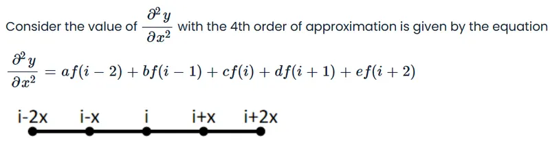
Consider Taylor Table for central difference

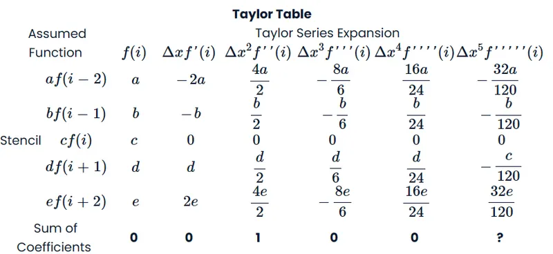
Writing the coefficients in the form of a matrix we get

2. Skewed right-sided difference

The number of Nodes required for 4th order approximation of a second-order derivative can be given by the equation.

The number of Nodes required for 4th order approximation of a second-order derivative can be given by the equation

N=P+QN=P+Q where

NN is the number of nodes

QQ is the order of derivative

PP is the order of approximation

So, here we need 6 nodes in order to find the 2nd order derivative with the 4th order of approximation.

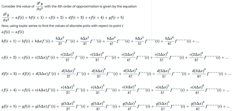
Adding the LHS and RHS of the above equations we get

af(i)+bf(i+1)+cf(i+2)+df(i+3)+ef(i+4)+gf(i+5)=f(i)[a+b+c+d+e+g]+Δxf'(i)[b+2c+3d+4e+5g]+Δx2f''(i)[b2+4c2+9d2+16e2+25g2]+Δx3f'''(i)[b6+8c6+27d6+64e6+125g6]+Δx4f''''(i)[b24+16c24+81d24+256e24+625g24]+Δx5f'''''(i)[b120+32c120+243d120+1024e120+3125g120]

In the above equations, we want only the coefficients of Δx2f''(i)Δx2f′′(i) and we assume the coefficient to be one and for the remaining terms we assume the coefficients to be zero.

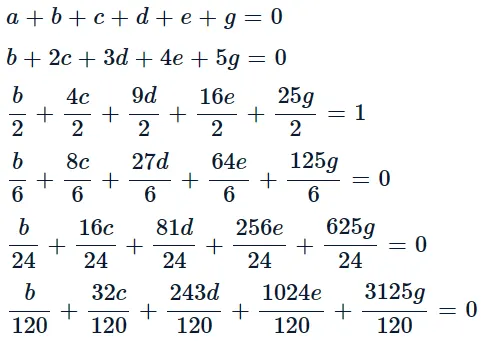
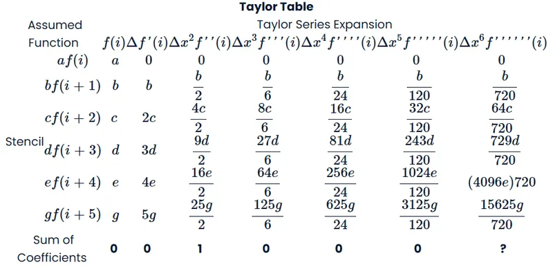
Writing the coefficients in the form of a matrix we get

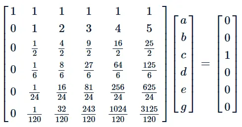
Now we can write the equation using the Taylors Table as

3. Skewed left-sided difference

The number of Nodes required for 4th order approximation of a second-order derivative can be given by the equation

N=P+QN=P+Q where

NN is the number of nodes

QQ is the order of derivative

PP is the order of approximation

So, here we need 6 nodes in order to find the 2nd order derivative with the 4th order of approximation.

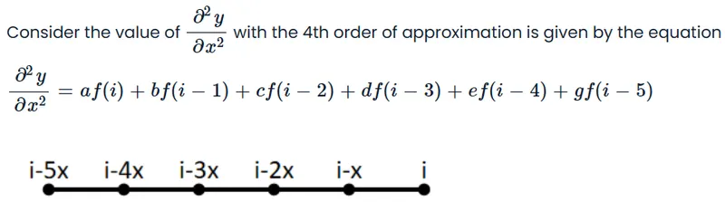
Consider Taylor Table for left-sided difference

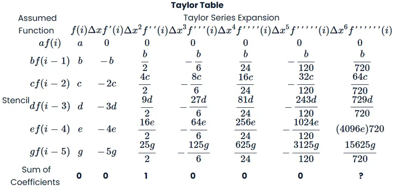
Writing the coefficients in the form of a matrix we get

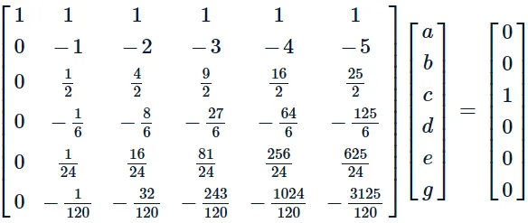
Solving using MATLAB to find the values of the coefficients

Now we can write the equation using the Taylors Table as

MATLAB CODE

clear all
close all
clc
% Finding the coefficients
% For Central difference
A_1=[1, 1, 1, 1, 1;-2, -1, 0, 1, 2;4/2, 1/2, 0, 1/2, 4/2;-8/6, -1/6, 0, 1/6, 8/6;16/24, 1/24, 0, 1/24, 16/24];
B_1=[0;0;1;0;0];
X_1=A_1\B_1

%For Skewed right-sided difference
A_2=[1 1 1 1 1 1;0 1 2 3 4 5;0 1/2 4/2 9/2 16/2 25/2;0 1/6 8/6 27/6 64/6 125/6;0 1/24 16/24 81/24 256/24 625/24;0 1/120 32/120 243/120 1024/120 3125/120];
B_2=[0;0;1;0;0;0];
X_2=A_2\B_2

% For Skewed left-sided difference
A_3=[1 1 1 1 1 1;0 -1 -2 -3 -4 -5;0 1/2 4/2 9/2 16/2 25/2;0 -1/6 -8/6 -27/6 -64/6 -125/6;0 1/24 16/24 81/24 256/24 625/24;0 -1/120 -32/120 -243/120 -1024/120 -3125/120];
B_3=[0;0;1;0;0;0];
X_3=A_3\B_3

% Finding the analytical derivative
%DEfine x as 60degree
x=pi/3;
% f(x) = exp(x)*cos(x)
analytical_soln = -2*sin(x)*exp(x)

% Finding the approximate solution
% Define dx
dx = linspace(pi/4000,1.5*pi,50); % taking a reasonable random number 50

% Finding Central difference approximation
a_1 = -0.0833;
b_1 = 1.3333;
c_1 = -2.5;
d_1 = 1.3333;
e_1 = -0.0833;
central_aprx = (a_1.*exp(x-2.*dx).*cos(x-2.*dx)+b_1.*exp(x-dx).*cos(x-dx)+c_1.*exp(x).*cos(x)+d_1.*exp(x+dx).*cos(x+dx)+e_1.*exp(x+2.*dx).*cos(x+2.*dx))./((dx).^2);

% Finding Skewed right-sided approx
a_2 = 3.75;
b_2 = -12.8333;
c_2 = 17.8333;
d_2 = -13.00;
e_2 = 5.0833;
g_2 = -0.8333;
skew_right_aprx = (a_2.*exp(x).*cos(x)+b_2.*exp(x+dx).*cos(x+dx)+c_2.*exp(x+2.*dx).*cos(x+2.*dx)+d_2.*exp(x+3.*dx).*cos(x+3.*dx)+e_2.*exp(x+4.*dx).*cos(x+4.*dx)+g_2.*exp(x+5.*dx).*cos(x+5.*dx))./((dx).^2);

% Finding Skewed left-sided approx
a_3 = 3.75;
b_3 = -12.8333;
c_3 = 17.8333;
d_3 = -13.00;
e_3 = 5.0833;
g_3 = -0.8333;
skew_left_aprx = (a_3.*exp(x).*cos(x)+b_3.*exp(x-dx).*cos(x-dx)+c_3.*exp(x-2.*dx).*cos(x-2.*dx)+d_3.*exp(x-3.*dx).*cos(x-3.*dx)+e_3.*exp(x-4.*dx).*cos(x-4.*dx)+g_3.*exp(x-5.*dx).*cos(x-5.*dx))./((dx).^2);

% Finding Errors
% Center approx error
error_central = abs(analytical_soln - central_aprx);
% Skewed right-sided error
error_right = abs(analytical_soln - skew_right_aprx);
% Skewed left-sided error
error_left = abs(analytical_soln - skew_left_aprx);

%Plot the error vs dx graph
loglog(dx,error_central,dx,error_right,dx,error_left)
xlabel('increasing dx grid spacing')
ylabel('Truncation error')
legend('Central Approximation Error','Skew-right error','Skew-left error')
title('truncation error behavious for different approximation')

RESULTS

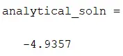
Analytical Result

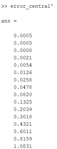
Central error

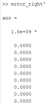
Skew right error

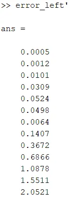
Skew left error

Log-Log graph

CONCLUSION

Following points can be concluded:-

The central scheme is most accurate among the three

Approximation becomes unstable for very high or lox value of dx, this is due combination of various errors like oundoff error, residual error and truncation error.

The most stable range for approximation is from 0.1 - 0.01.

Q. Why skewed scheme is useful? What can a skewed scheme do that a central differencing scheme cannot?

The central differencing requires information from both side from point-to-point, wheareas applications where answer is predicted using the boundary conditions skewed scheme will be the most usefull as we will have only one direction to follow.