Week 3.5 - Deriving 4th order approximation of a 2nd order derivative using Taylor Table method

[0; 0; 1; 0; 0; 0];

From this we can calculate a,b,c,d and e and then the aproximation with Skewed right-sided difference can be calculated.

No.of nodes from stencil, N = 6

Order of derivative, Q = 2

From hint(ii)

The derived equations in the matrix form

Coefficient Matrix, A =

% Program for Week 3.5 - Deriving 4th order approximation of a 2nd order derivative using Taylor Table method
clear all 
close all
clc

%Initialize x and dx
x = pi/3;
dx = linspace(pi/40,pi/4000,20);

% Given analytical function
% exp(x)*cos(x)

analytical_derivative = -2*exp(x)*sin(x)

% 4th order approximations of the second-order derivative

% 1. Central difference
for i = 1:length(dx) % calculating error over different values of dx
    central_diff_error(i) = abs(central_diff_approximation(x,dx(i))-analytical_derivative); % Absolute error calculation
end

% 2.Skewed right sided difference
for i = 1:length(dx) % calculating error over different values of dx
    skewed_righthanded_error(i) = abs(skewed_righthanded_approximation(x,dx(i))-analytical_derivative); % Absolute error calculation
end

% 3.Skewed left sided difference
for i = 1:length(dx) % calculating error over different values of dx
    skewed_lefthanded_error(i) = abs(skewed_lefthanded_approximation(x,dx(i))-analytical_derivative); % Absolute error calculation
end

% Plotting of absolut error for the three schemes
figure(1)
loglog(dx,central_diff_error)
hold on
loglog(dx,skewed_righthanded_error,'r')
hold on
loglog(dx,skewed_lefthanded_error,'g')
% giving proper labels
xlabel('dx')
ylabel('Absolte error')
legend('Central difference error','Skewed right hand error','Skewed left hand error')

PROGRAM EXPLANATION:

• Line 7,8: Initializes the x and dx for calculations.
• Line 11: Indicate the given equation whose second order derivative has to be calculated using the three schemes of approximations.
• Line 13: Calculates the analytical second order derivative for the given function.
• Line 18-20: Using for loop to calculate the absolute error for central difference scheme for all the values of dx.
• Line 19: Calulates the absolute error using central_diff_approximation() and stores it in central_diff_error() array.
• Line 23-25: Using for loop to calculate the absolute error for skewed right sided difference scheme for all the values of dx.
• Line 24: Calulates the absolute error using skewed_righthanded_approximation() and stores it in skewed_righthanded_error() array.

• Line 28-30: Using for loop to calculate the absolute error for skewed left sided difference scheme for all the values of dx.
• Line 29: Calulates the absolute error using skewed_lefthanded_approximation() and stores it in skewed_lefthanded_error(i) array.
• Line 33-38: Plots the graph of absolute error against dx for all three schemes in different colours.
• Line 40-42: Gives the proper labeling to the graphs for easy understanding.

FUNCTIONS USED:

central_diff_approximation()

function out = central_diff_approximation(x,y)

A_cd = [1      1     1    1      1; 
       -2     -1     0    1      2; 
        4/2    1/2   0    1/2    4/2; 
       -8/6   -1/6   0    1/6    8/6; 
        16/24  1/24  0    1/24   16/24]; % Coefficient matrix for central differencing

B_cd = [0; 0; 1; 0; 0]; % Constant Matrix for central differencing

X_cd = A_cd\B_cd; % Calculated matrix which gives values of a,b,c,d,e for central differencing

%terms correspond to a,b,c,d and e in the derived equation
M_cd = [exp(x-2*y)*cos(x-2*y) exp(x-y)*cos(x-y) exp(x)*cos(x) exp(x+y)*cos(x+y) exp(x+2*y)*cos(x+2*y)]; 

out = (M_cd*X_cd)/y^2;

%out = X_cd(1)*exp(x-2*y)*cos(x-2*y)+X_cd(2)*exp(x-y)*cos(x-y)+X_cd(3)*exp(x)*cos(x)+X_cd(4)*exp(x+y)*cos(x+y)+X_cd(5)*exp(x+2*y)*cos(x+2*y)
end

skewed_righthanded_approximation()

function out = skewed_righthanded_approximation(x,y)

A_sr = [1      1       1       1       1        1;
        0      1       2       3       4        5;
        0      1/2     4/2     9/2     16/2     25/2;
        0      1/6     8/6     27/6    64/6     125/6;
        0      1/24    16/24   81/24   256/24   625/24;
        0      1/120   32/120  243/120 1024/120 3125/120]; % Coefficient matrix for Skewed right sided difference

B_sr = [0; 0; 1; 0; 0; 0]; % Constant Matrix for Skewed right sided difference

X_sr = A_sr\B_sr; % Calculated matrix which gives values of a,b,c,d,e for Skewed right hand difference

%terms correspond to a,b,c,d,e and g in the derived equation
M_sr = [exp(x)*cos(x) exp(x+y)*cos(x+y) exp(x+2*y)*cos(x+2*y) exp(x+3*y)*cos(x+3*y) exp(x+4*y)*cos(x+4*y) exp(x+5*y)*cos(x+5*y)];

out = (M_sr*X_sr)/y^2;

end

skewed_lefthanded_approximation()

function out = skewed_lefthanded_approximation(x,y)

A_sl = [1           1          1         1        1       1;
       -5          -4         -3        -2       -1       0;
        25/2        16/2       9/2       4/2      1/2     0;
       -125/6      -64/6      -27/6     -8/6     -1/6     0;
        625/24      256/24     81/24     16/24    1/24    0;
        3125/120   -1024/120   -243/120 -32/120  -1/120  0]; % Coefficient matrix for Skewed left sided difference

B_sl = [0; 0; 1; 0; 0; 0]; % Constant Matrix for Skewed left sided difference

X_sl = A_sl\B_sl; % Calculated matrix which gives values of a,b,c,d,e for Skewed left sided difference

%terms correspond to a,b,c,d,e and g in the derived equation
M_sl = [exp(x-5*y)*cos(x-5*y) exp(x-4*y)*cos(x-4*y) exp(x-3*y)*cos(x-3*y) exp(x-2*y)*cos(x-2*y) exp(x-y)*cos(x-y) exp(x)*cos(x)];

out = (M_sl*X_sl)/y^2;


end

FUNTION CODE EXPLANATION:

• Line 1: Creates a funtion and the out as an output for the funtion and takes x, y as inputs where y=dx(i).
• Line 3-7/8: Initializes the coefficient matrix,A obtained from the derived equations for that particular scheme.
• Line 9/10: Initializes the constant matrix,B for the scheme.
• Line 11/12: The matrix, X which consists of the variables is calculted from the formula X = A\B.
• Line 13/14: Initialize M matrix with the terms corresponding to a,b,...
• Line 23-25: Calculates the numerical approximations for the scheme and store it in the variable out.

OUTPUT:

OUTPUT EXPLANATION:

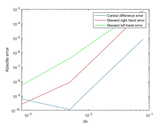
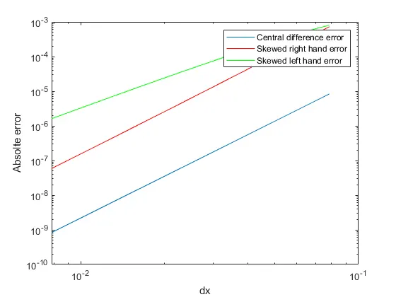
• The graph shows the error decreases with decrease of dx value. Also, central difference error < skewed right sided error ~ skewed left sided error.
• Also, if the value of dx is loweres significantly, it causes a round off error which is why the graph looks like that.
• So, changing the values of dx the following output can be obtained.

In your own words, describe why a skewed scheme is useful? What can a skewed scheme do that a CD scheme cannot?

• In most cases, we would have the information in one direction and the characteristics has to be calculated. Here skewed schemes can be useed to calculate them numerically.
• Also, at the boundary, we will have only one sided information and central difference cannot be used to find the boundary conditions because there is no information beyond the boundary.