Week 3 - Solving second order ODEs

GOALS:

• Program to simulate the motion of the pendulum with the given inputs and conditions.
• Using ode45 function to solve the ODE that represents the motion of the simple pendulum.
• Create an animation for the motion of the pendulum.
• Write the animation onto a video file and upload it in the youtube.

MAIN PROGRAM:

% Program to solve ODE of a simple pendulum
% ALso includes the code to animate the pendulum 
clear all
close all
clc

% Inputs of the pendulum
l = 1; % length of the pendulum in m
m = 1; % mass of the pendulum in Kg
b = 0.05; % damping coefficient
g = 9.81; % acceleration due to gravity in m/s^2

% Initial conditions
% angular displacement = 0 and angular velocity = 3 rad/s at t = 0
theta_0 = [0;3];

% Time plots
t_span = linspace(0,20,500);

% Solving ODE using function
[t, result] = ode45(@(t,theta) pendulum_func(t, theta, l, m, b, g),t_span,theta_0);

% Plotting the result

% Plot of angular displacement with time
figure(1)
plot(t, result(:,1), 'Color','r')
hold on
grid on

% Plot of angular velocity with time
plot(t, result(:,2), 'Color','b')
xlabel('Time in s')
legend('Angular Displacement','Angular Velociity')
grid on
hold off

% Animation of the pendulum

% Position of the Bob
x_bob = sin(result(:,1));
y_bob = -cos(result(:,1));

ct =1;
figure(2)
for i = 1:length(t)
    clf
    plot([-1.5,1.5],[0,0],'LineWidth',10,'Color','b') % Wall from which the pendulum is hung
    hold on
    plot([0,0],[0,-1.5],'LineStyle','--','Color','k') % Central line
    hold on
    plot(x_bob,y_bob,'LineStyle',':','Color','r') % Bob trace
    hold on
    
    % String of the pendulum
    plot([0,x_bob(i)],[0,y_bob(i)],'LineWidth',3,'LineStyle','-','Color','g')
    
    % Bob of the pendulum
    plot(x_bob(i),y_bob(i),'r-o','MarkerSize',30,'MarkerFaceColor','r')
    
    %Joint of pendulum to the wall
    plot(0,0,'y-o','MarkerSize',10,'MarkerFaceColor','y')
    
    %plot(x_bob(i),y_bob(i),'LineStyle',':','Color','r')
    % Axes limits
    axis([-1.5 1.5 -1.5 0])
    %pause(0.05)
    M(ct) = getframe(gcf);
    ct = ct + 1;
end

%code to convert the saved plot into a video
movie(M)
videofile = VideoWriter('Pendulum_Animation.avi','Uncompressed AVI');
open(videofile)
writeVideo(videofile,M)
close(videofile)

FUNCTION USED:

function [dtheta_dt] = pendulum_func(t, theta, l, m, b, g)

    theta1 = theta(1);
    theta2 = theta(2);
    
    % Converting of 2nd order differrentaial to 1st order differential
    % equations
    dtheta1_dt = theta2;
    dtheta2_dt = -(b/m)*theta2-(g/l)*theta1;
    
    dtheta_dt = [dtheta1_dt; dtheta2_dt];

end

CODE EXPLANATION:

• Line 7-11: In these lines the inputs of the pendulum are given in SI units.
• Line 15: The initial angular displacement and velocity at t = 0 are initialized to theta_0.
• Line 18: The pendulum motion is simulated for 20 sec with 500 values taken for time t_span from 0 to 20s.
• Line 21: ode45 solver is used to solve the ODE of the pendulum.
  • ode45 with inputs
    • @(t,theta) - meaning it is a function of t and theta.
    • pendulum_func(t, theta, l, m, b, g) - values of dtheta_dt are obtaion from this fuction.
    • t_span - gives the time limits for the integration.
    • theta_0 - initial conditions for the integration.
  • The results are stored in [t, result].
• Line 23-26: Plotting the angular displacement and the angular velocity of the pendulum for 20s in Figure 1.
• Line 41-42: The x- and y-postion of the bob is obtained using the triganometric functions.
• Line 46: for loop is used to iterate the code that captures the each postion of the pendulum for particular time t. The loop is iterated for all the values of t.
• Line 47: clf is used at the start to clear the any previous frame plotted so that the new frame can be plotted.
• Line 48: The wall from which the pendulum hung is plotted with colour blue and a linewidth of 10.
• Line 50: The central dotted line is plotted.
• Line 52: The positions of the bob is drawn as a dotted line on the plot with red colour.
• Line 56: The string of the pendulum is plotted in green colour with linewidth of 3.
• Line 59: The bob of the pendulum is created using the marker command.
• Line 62: The joint of the pendulum to the wall is plotted in yellow colour.
• Line 66: The axes limits for the plot are given here.
• Line 68: The frame created is then stored into n array M using getframe() funtion.
• Line 72-77: The array M is then converted into videofile.

FUNCTION CODE EXPLANATION:

• Line 1: The inputs of the funtion are t, theta, l, m, b, g which were all given parameters. The results are then stored in [dtheta_dt].
• Line 8-9: Converts the second order differential equation to first order ODEs.
• Line 11: Stores the equations into [dtheta_dt] matrix.

OUTPUTS:

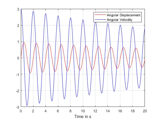
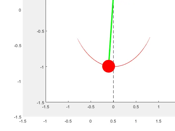
OUTPUT 1 EXPLANATION:

• The angular dispacement is o rad at time t=0 as given by the input parameters.
• The angular veloctity is 3 rad/sec as stated.
• Both graphs slowly dampens with time indicating the slowing of the pendulum over time because of the damping to the pendulum.

OUTPUT 2 EXPLANATION:

• The second output shows the postion of the pendulum at a particular time t.

VIDEO FILE LINK:

https://youtu.be/QsBQpFCeJYE