Challenge

Week 4.1 - Genetic Algorithm

KKalidindi Prasad Raju22 Jun 2022

OBJECTIVES:

Understand the concept of optimization and optimizing a function using genetic algorithm in Matlab.
Explain the concept of genetic algorithm and the syntax of ga in Matlab.
Learn about the stalgamite funtion and the ways to optimize it.
Program a code to optimize the given stalgamite function and find its global maximum using ga.
Plot the graphs for F-maximum vs No.of iterations for the 3 studies performed.

GENETIC ALGORITHM:

Genetic Alogithm is a concept of optimization which genrates a population to find the best solution. It is based on the concept of evolution where the child is generated from parents that are genetically evolved.
This process of generating population repeats until an optimum solution is reached.

Syntax of ga in Matlab:

opt_value = ga(func, nvars, A, b, Aeq, beq, lb, ub, nonlcon, options)

func - is the function that needs to be optimized.

nvars - no.of variables in the given funtion.

A,b - are linear inequality constraints of the function

Aeq,beq - are linear inequality constraints

lb, ub - are lower and upper bounds for the optimizing points

nonlcon - are nonlinear constraints

options - are options that can be given to the ga over its normal calculation limits.

Stopping Criteria:

These are the criteria available in GA to stop optimizing once the criteria is reached.

Maxgenerations: The GA stops after the no.of generation reaches the Maxgenerations value.
MaxTime: It stops after a predtermined MaxTime ends.
FitnessLimit: When the value of the fitness function of the best point is less than or equal to the given FitnessLImit, the algorithm stops automatically.
MaxStallGenerations: When the average relative change in the function over the amount MaxStallGenerations is less than the given Fitness tolerance then the GA stops.
MaxStallTime: The GA stops when there is no change in the objecctive function for MaxStallTime seconds.
FunctionTolerance: The GA stops when the average relative change in the function over the amount MaxStallGenerations is less than the given Fitness tolerance.

MAIN CODE:

% Program about ga Week 4.1 challenge
clear all 
close all
clc

% Defining the search space
x = linspace(0,0.6,150);
y = linspace(0,0.6,150);

% creating a 2D mesh
[xx yy] = meshgrid(x,y);

%Evaluating stalgamite function
for i = 1:length(x)
    for j = 1:length(y)
        input_vector(1) = xx(i,j);
        input_vector(2) = yy(i,j);
        f(i,j) = stalagamite(input_vector);
    end 
end

%surfc(x,y,f)
%shading interp
%[inputs, fval] = ga(@stalagamite, 2)
tic
% Study 1 - Satistical Study
numcases = 50;
for i = 1:numcases
    [inputs, fopt(i)] = ga(@stalagamite, 2);
    xopt(i) = inputs(1);
    yopt(i) = inputs(2);
end
study1_time = toc

figure(1)
subplot(2,1,1)
hold on
surfc(x,y,-f)
shading interp
plot3(xopt,yopt,-fopt,'Marker','o', 'MarkerSize',5,'MarkerFaceColor','r')
title('Unbounded inputs')
subplot(2,1,2)
plot(-fopt)
xlabel('No.of Iterations')
ylabel('Function Maximum')

tic
% Study 2 - Adding upper and lower bounds to study 1
numcases = 50;
for i = 1:numcases
    [inputs, fopt(i)] = ga(@stalagamite, 2,[],[],[],[],[0;0],[0.4;0.4]);
    xopt(i) = inputs(1);
    yopt(i) = inputs(2);
end
study2_time = toc

figure(2)
subplot(2,1,1)
hold on
surfc(x,y,-f)
shading interp
plot3(xopt,yopt,-fopt,'Marker','o', 'MarkerSize',5,'MarkerFaceColor','r')
title('Bounded inputs')
subplot(2,1,2)
plot(-fopt)
xlabel('No.of Iterations')
ylabel('Function Maximum')

tic
% Study 3 - Increasing the GA iterations
options = optimoptions('ga');
options = optimoptions(options, 'PopulationSize',150);

numcases = 50;
for i = 1:numcases
    [inputs, fopt(i)] = ga(@stalagamite,2,[],[],[],[],[0;0],[0.4;0.4],[],[],options);
    xopt(i) = inputs(1);
    yopt(i) = inputs(2);
end
study3_time = toc

figure(3)
subplot(2,1,1)
hold on
surfc(x,y,-f)
shading interp
plot3(xopt,yopt,-fopt,'Marker','o', 'MarkerSize',5,'MarkerFaceColor','r')
title('Bounded inputs with population size increase')
subplot(2,1,2)
plot(round(-fopt))
xlabel('No.of Iterations')
ylabel('Function Maximum')

FUNCTION USED:

function f = stalagamite(input_vector)
    x = input_vector(1);
    y = input_vector(2);

    f1x = (sin(5.1*pi*x + 0.5))^6;
    f1y = (sin(5.1*pi*y + 0.5))^6;

    f2x = exp(((-4*log(2)*(x-0.0667)^2))/(0.64));
    f2y = exp(((-4*log(2)*(y-0.0667)^2))/(0.64));

    f = -f1x*f1y*f2x*f2y;
end

CODE EXPLANATION:

Line 7-8: Defines the search space for the stalgamite function.
Line 11: Creates a mesh grid of the defined search space.
Line 14-20: Using nested for loop to initialize the values of meshgrid xx, yy to the input_vector. Also calculating the value of the stalgamite function.
Line 28-32: Claculating the optimum function values and optimum points using ga and assigning them to variables over the given no.of iterations. In this study, the optimum values are generated without any bounded limits.
Line 25,33: Using tic and tac commands to calculte the time taken to find the optimum values for the given no.of iterations.
Line 36,42: subplot function is used to plot two graphs in one figure.
Line 38: Plots the function in the given search space. "-" sign is used to convert the negative value of the function maximum to postive.
Line 39: shading interp is used for smooth shading of the function.
Line 40: plot3() function is used to plot the optimum function values in 3D and connecting them using line.
Line 41: gives the title to the plot.
Line 43: plots the optimum function value for each iteration.
Line 44,45: labels the x-, y- axis of the plot.

Line 49-54: Claculating the optimum function values and optimum points using ga and assigning them to variables over the given no.of iterations. In this study, the optimum values are generated with the bounded limits of x from 0 to 0.4 and y from 0 to 0.4.
Line 47,55: Using tic and tac commands to calculte the time taken to find the optimum values for the given no.of iterations.
Line 58,64: subplot function is used to plot two graphs in one figure.
Line 60: Plots the function in the given search space. "-" sign is used to convert the negative value of the function maximum to postive.
Line 61: shading interp is used for smooth shading of the function.
Line 62: plot3() function is used to plot the optimum function values in 3D and connecting them using line.
Line 63: gives the title to the plot.
Line 65: plots the optimum function value for each iteration.
Line 66,67: labels the x-, y- axis of the plot.

Line 71-72: Increases the population size to 150 instead of 100 which is default for ga
Line 74-90: Claculating the optimum function values and optimum points using ga and assigning them to variables over the given no.of iterations. In this study, the optimum values are generated with the bounded limits of x from 0 to 0.4 and y from 0 to 0.4 and a population size of 150.
Line 69,80: Using tic and tac commands to calculte the time taken to find the optimum values for the given no.of iterations.
Line 83,89: subplot function is used to plot two graphs in one figure.
Line 85: Plots the function in the given search space. "-" sign is used to convert the negative value of the function maximum to postive.
Line 86: shading interp is used for smooth shading of the function.
Line 87: plot3() function is used to plot the optimum function values in 3D and connecting them using line.
Line 88: gives the title to the plot.
Line 90: plots the optimum function value for each iteration.
Line 91,92: labels the x-, y- axis of the plot.

FUNCTION EXPLANATION:

Line 2-3: Assigning input_vector values to x and y.
Line 5-9: Calculates the four values needed for calculating stalagmite function.
Line 11: Claculates the values of the stalagmite function for the given x and y. "-" sign is used to calculate global maxima instead of global minima. It is because ga generally can only calculte function minima.

OUTPUT:(excluding optimization terminated lines)

study1_time =

9.9314

study2_time =

8.2268

study3_time =

14.9308

OUTPUT EXPLANATION:

study1_time > study2_time because it takes more time to calculate optimum values in study 1 for calculating the values over the limit which are unnecessary.
study3_time > study2_time because it takes more time to calculate optimum values in study 3 due to its increased population size than study 2.

FIGURE 1:

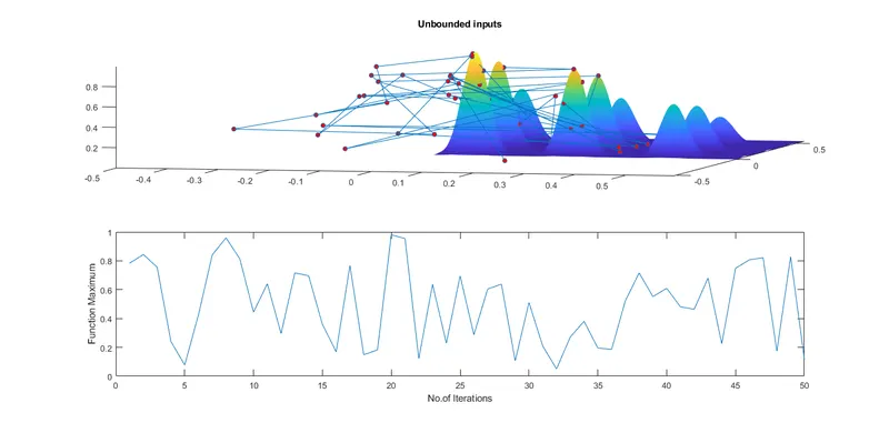
FIGURE 1 EXPLANATION:

The first plot shows the function maixima as a red marker at each iteration. Because no bounded limits are given the ga calculates the function maxima over the search area also.
The second plot shows the value of function maxima at each iteration. It shows the value of function maxima changes for each iteration. That is the reason to calculate the optimize value over iterations to check whether the calculated value is correct. Otherwise, its value changes each time the program runs. So, to find the actual function maxima bounded limits can be used.

FIGURE 2:

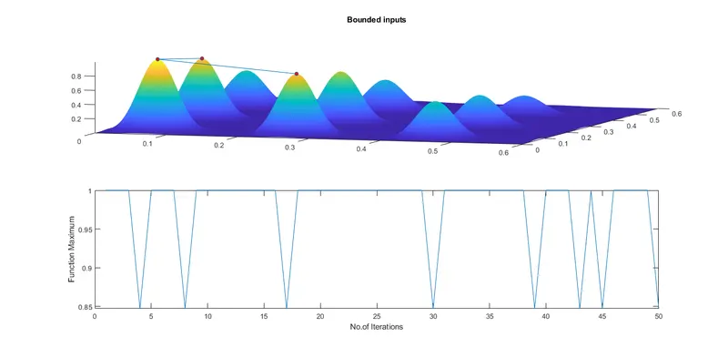
FIGURE 2 EXPLANATION:

With the bounded limits the ga calculates the optimized fuction value within the given limits.
Still, the function maxima is shown to be between three points. To find the actual function maxima, the population size can be increased.

FIGURE 3:

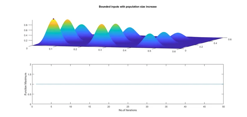
FIGURE 3 EXPLANATION:

By increasing the population size to 150, the ga was able to calculte the actaul function maxima which does not change with the no.of iterations.

Week 4.1 - Genetic Algorithm

Ship work like this
in your own course.

Talk to a career counsellor

Ship work like thisin your own course.

Talk to a career counsellor

Ship work like this
in your own course.