Week 3.5 - Deriving 4th order approximation of a 2nd order derivative using Taylor Table method

OBJECTIVE;

To Derive the following 4th order approximations of the second-order derivative. Central difference, Skewed right-sided difference, Skewed left-sided difference and will be comapring the skewed diiferences with one another and with the analytical derivative.

CENTRAL DIFFERENCING SCHEME:

In central differencing we will be taking the references from both sides of the function symmetrically to derive the order of approximations.

here no of nodes = p+q-1

where p = order of derivative (2)

q = order of error approxmations (4)

so no of nodes = 5

DERIVATION:

To derive a fourth order approximation for the second order derivative.

`(delta^2u)/(deltax^2) = (af(i-2) + bf(i-1) + cf(i )+ df(i+1) + ef(i+2))/(dx^2)`

taylor series for each term is found out and set in taylor table.

taylor series for

`af(i-2) = a(f(i) - (f'(i)2dx)/(1!)+(f'''(i)4dx^2)/(2!)+(f''''(i)8dx^3)/(3!)+(f''''(i)16dx^4)/(4!)...`(1)

taylor table

f''(i)`dx^2`	f(i)	f'(i)dx	`f''(i)dx^2`	`f'''(i)dx^3`	`f''''(i)dx^4`
af(i-2)	a	-2a	2a	`-(4a)/3`	`(2a)/3`
bf(i-1)	b	-b	`b/2`	`(-b)/6`	`b/24`
cf(i)	c	0	0	0	0
df(i+1)	d	d	`d/2`	`(d)/6`	`d/24`
ef(i+2)	e	2e	2e	`(4e)/3`	`(2e)/3`
sum of co_efficients	0	0	1	0	0

with the help of taylor table we can find the coefficients by using the matrix multiplication ;

A.X = B as we know

`[[1 1 1 1 1], [-2 -1 0 1 2], [2 1/2 0 1/2 2],[-4/3 -1/6 0 1/6 -4/3],[2/3 1/24 0 1/24 2/3] ]``((a), (b), (c), (d),( e))`=`((0),(0),(1),(0),(0))`

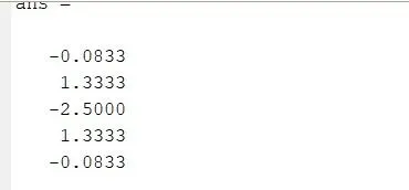
a = -0.0833

b= 1.3333

c= -2.5000

d = 1.333

e = -0.0833

substituting these values in equation (1)

`(delta^2u)/(deltax^2) = (-0.0833f(i-2) + 1.333f(i-1) + 2.5000f(i )+ 1.333f(i+1) + -0.0833f(i+2))/(dx^2)`

SKEWED LEFT HAND SCHEME:

no of nodes = p +q

p - order of derivative

q - order of error approximations

nodes = 6

deriving a fourth order approximation fro deriving a second order derivative. The formula goes into

`(delta^2u)/(deltax^2) = (af(i-5) + bf(i-4) + cf(i-3 )+ df(i-2) + ef(i-1)+gf(i))/(dx^2)`......(2)

expanding all the terms using taylor table

`deltax^2`f(i)	f(i)	f'(i)dx	`f''(i)deltax^2`	`f'''(i)deltax^3`	`f''''(i)deltax^4`	`f'''''(i)deltax^5`
af(i-5)	a	-5a	`(25a)/2`	`(-125a)/6`	`(625a)/24`	`(-3125a)/120`
bf(i-4)	b	-4b	`(16b)/2`	`(-64b)/6`	`(256b)/24`	`(-1024b)/120`
cf(i-3)	c	-3c	`(9c)/2`	`(-27c)/6`	`(81c)/24`	`(-243c)/120`
df(i-2)	d	-2d	`(4d)/2`	`(-8d)/6`	`(16d)/24`	`(-32e)/120`
ef(i-1)	e	-e	`e/2`	`-e/6`	`e/24`	`-e/120`
gf(i)	g	0	0	0	0	0
sum of co_efficients	0	0	1	0	0	0

with the help of taylor table we can find the coefficients by using the matrix multiplication ;

A.X = B as we know

`[[1 1 1 1 1 1], [-5 -4 -3 -2 -1 0], [25/2 16/2 0 9/2 1/2 0],[-125/6 -64/6 -27/6 -8/6 -1/6 0],[625/24 256/24 81/24 16/24 1/24 0],[-3125/120 -1024/120 -243/120 -32/120 -1/120 0 ] ]``((a), (b), (c), (d),( e),(g))`=`((0),(0),(1),(0),(0),(0))`

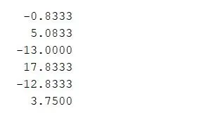
a= -0.8333

b= 5.0833

c = -13

d= 17.8333

e = -12.8333

g=3.75

substituting these values in equation (2)

`(delta^2u)/(deltax^2) = (-0.8333f(i-5) + 5.0833f(i-4) + -13f(i-3 )+ 17.8333f(i-2) + -12.8333f(i-1)+3.75f(i))/(dx^2)`

RIGHT SKEWED SCHEME:

no fo nodes = p+q

p =order of the derivative

q = order of error approximations. so no of nodes for right skewed scheme is 6

deriving a fourth order approximation fro deriving a second order derivative. The formula goes into

`(delta^2u)/(deltax^2) = (af(i) + bf(i+1) + cf(i+2 )+ df(i-+3) + ef(i+4)+gf(i+5))/(dx^2)`......(3)`

expanding all the terms using taylor table

`dx^2f''(i)`	f(i)	f'(i)dx	`f''(i)dx^2`	`f'''(i)dx^3`	`f''''(i)dx^4`	`f'''''(i)dx^5`
af(i)	a	0	0	0	0	0
bf(i+1)	b	b	`b/2`	`b/6`	`b/24`	`b/120`
cf(i+2)	c	2c	`(4c)/2`	`(8c)/6`	`(16c)/24`	`(32c)/120`
df(i+3)	d	3d	`(9d)/2`	`(27d)/6`	`(81d)/24`	`(243d)/120`
ef(i+4)	e	4e	`(16e)/2`	`(64e)/6`	`(256e)/24`	`(1024e)/120`
gf(i+5)	g	5g	`(25g)/2`	`(125g)/6`	`(625g)/24`	`(3125g)/120`
sum of co_efficients	0	0	1	0	0	0

with the help of taylor table we can find the coefficients by using the matrix multiplication ;

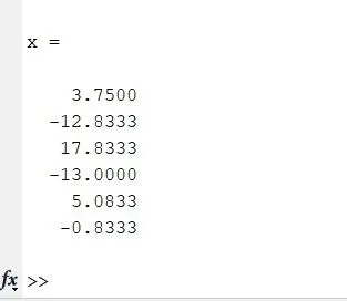
A.X = B as we know

THE CODE;

clear all
close all
clc

%function =  exp(x)*cos(x)
%f''(x) = -2*exp(x)*sin(x)

% numerical disretization for a range of dx
x=pi/3;
dx= linspace(pi/40,pi/4000,20);

for i=1:length(dx)
    central_differencing_scheme(i) = center_fourth_order(x,dx(i));
    right_skewed_scheme(i) = rightskewed_fourth_order(x,dx(i));
    left_skewed_scheme(i) = leftskewed_fourth_order(x,dx(i));
    
   
end

%plotting
% lolog command for finite graphical view
figure(1)
loglog(dx,central_differencing_scheme);
hold on 
loglog(dx,right_skewed_scheme);
hold on
loglog(dx,left_skewed_scheme);
xlabel('range dx')
ylabel('truncation errors')
legend('centraldifference_fourth_order_error','right_skewed_fourth_order_error','left_skewed_fourth_order_error')

FUNCTION FOR CENTRAL DIFFERENCING SCHEME

function center_fourth_order_error = center_fourth_order(x,dx)
%function = exp(x)*cos(x)
%f''(x) = -2*exp(x)*sin(x)

analytical_derivative = -2*exp(x)*sin(x)

%numerical derivative
center_fourth_order =  (((-0.0833)*((exp(x-(2*dx)))*(cos(x-(2*dx)))))+((1.3333)*((exp(x-dx))*(cos(x-dx))))-((2.5000)*((exp(x))*(cos(x))))+((1.3333)*((exp(x+dx))*(cos(x+dx))))-((0.0833)*((exp(x+(2*dx)))*(cos(x+(2*dx))))))/(dx^2);

%error
center_fourth_order_error = abs(center_fourth_order-analytical_derivative);
end

FUNCTION FOR LEFT SKEWED

function leftskewed_fourth_order_error  = leftskewed_fourth_order(x,dx)
%function = exp(x)*cos(x)
%f''(x) = -2*exp(x)*sin(x)

analytical_derivative = -2*exp(x)*sin(x)

%numerical derivative
leftskewed_fourth_order = (((-0.8333)*((exp(x-(5*dx)))*(cos(x-(5*dx)))))+((5.0833)*((exp(x-(4*dx)))*(cos(x-(4*dx)))))-((13.0000)*((exp(x-(3*dx)))*(cos(x-(3*dx)))))+((17.8333)*((exp(x-(2*dx)))*(cos(x-(2*dx)))))-((12.8333)*((exp(x-dx))*(cos(x-dx))))+((3.7500)*((exp(x))*(cos(x)))))/(dx^2);

%error
leftskewed_fourth_order_error = abs(leftskewed_fourth_order-analytical_derivative);
end

FUNCTION FOR RIGHT SKEWED

function leftskewed_fourth_order_error  = rightskewed_fourth_order(x,dx)
%function = exp(x)*cos(x)
%f''(x) = -2*exp(x)*sin(x)

analytical_derivative = -2*exp(x)*sin(x)

%numerical derivative
rightskewed_fourth_order = (((3.7500)*((exp(x))*(cos(x))))-((12.8333)*((exp(x+dx))*(cos(x+dx))))+((17.8333)*((exp(x+(2*dx)))*(cos(x+(2*dx)))))-((13.0000)*((exp(x+(3*dx)))*(cos(x+(3*dx)))))+((5.0833)*((exp(x+(4*dx)))*(cos(x+(4*dx)))))-((0.8333)*((exp(x+(5*dx)))*(cos(x+(5*dx))))))/(dx^2);

%error
leftskewed_fourth_order_error= abs(rightskewed_fourth_order-analytical_derivative);
end

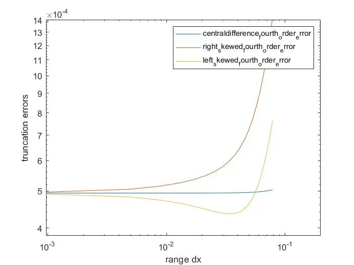
GRAPH

CONCLUSION:

central differencing scheme is summing for minimum error when compared to Left and right skewed schemes as it takes info from both the sides of the function but it has some limitaions where we cant use the central differencing scheme always .

WHY SKEWED SCHEME HAS SOME ADVANTAGES OVER CENTRAL DIFFERENCING SCHEME :

skewed scheme is better to use at deriving the derivatives at boundary layers and at some points where we can't use the central differencing scheme, eventhough when compared skewed and central differencing scheme has minor error variations between them