Deriving 4th order approximation of a 2nd order derivative using Taylor Table method

AIM

To derive and write a program for in MATLAB for fourth order approximation for second order derivative using central difference, skewed right-sided difference, and skewed left-sided difference schemes.

SCHEMES EQUATIONS AND COEFFICIENTS VALUES

1. Central Difference Scheme

The order of accuracy P = Number of nodes in the stencil N - order of derivative Q + 1 for symmetric/central schemes.
P=4 and Q=2
Number of nodes (N) = P+Q-1 = 4+2-1=5

Equation:
`(delta^2u)/(deltax^2) = (af(i-2)+bf(i-1)+cf(i)+df(i+1)+ef(i+2))/(Deltax^2)` -(1)

All terms in above mentioned equation 1 are expanded using taylor table method.

	f(i)	`Delta x`f'(i)	`Delta x^2`f''(i)	`Delta x^3`f'''(i)	`Delta x^4 f^(iv)`(i)	`Delta x^5 f^(v)`(i)	`Delta x^6 f^(vi)`(i)
af(i-2)	a	-2a	4a/2	-8a/6	16a/24	-32a/120	64a/240
bf(i-1)	b	-b	b/2	-b/6	b/24	-b/120	b/240
cf(i)	c	0	0	0	0	0	0
df(i+1)	d	d	d/2	d/6	d/24	d/120	d/240
ef(i+2)	e	2e	4e/2	8e/6	16e/24	32e/120	64e/240
`sum`of all coefficents	0	0	1	0	0	?	?

With the help of the taylor table, we can find the values of the coefficients.

Equations will be:

a+b+c+d+e=0
-2a-b+0+d+2e=0
4a/2 + b/2 + 0 +d/2 + 4e/2 = 1
-8a/6 -b/6 + 0 + d/6 + 8e/6 = 0
16a/24 + b/24 + 0 +d/24 +16e/24 = 0

In matrix form these equations become:

`[[1,1,1,1,1], [-2,-1,0,1,2], [4/2,1,0,1,4/2], [-8/6,-1/6,0,1/6,8/6], [16/24,1/24,0,1/24,16/24]]` * `[[a],[b],[c],[d],[e]]` = `[[0],[0],[1],[0],[0]]`

By using matlab, we get the values of the coefficients to be:
a= -0.0833
b= 1.3333
c= -2.5000
d= 1.3333
e= -0.0833

substituting these in equation 1, we get,
`(delta^2u)/(deltax^2) = (-0.0833f(i-2)+1.3333f(i-1)-2.5000f(i)+1.3333f(i+1)-0.0833f(i+2))/(Deltax^2)`

2. Skewed right-sided difference scheme

The order of accuracy P = Number of nodes in the stencil N + order of derivative Q
P=4 and Q=2
Number of nodes (N) = P+Q = 4+2=6

Equation:
`(delta^2u)/(deltax^2) = (af(i)+bf(i+1)+cf(i+2)+df(i+3)+ef(i+4)+gf(i+5))/(Deltax^2)` -(2)

from the above equation, usingt taylor table method, we get,

	f(i)	`Delta x`f'(i)	`Delta x^2`f''(i)	`Delta x^3`f'''(i)	`Delta x^4 f^(iv)`(i)	`Delta x^5 f^(v)`(i)
af(i)	a	0	0	0	0	0
bf(i+1)	b	b	b/2	b/6	b/24	b/120
cf(i+2)	c	2c	4c/2	8c/6	16c/24	32c/120
df(i+3)	d	3d	9d/2	27d/6	81d/24	243d/120
ef(i+4)	e	4e	16e/2	74e/6	256e/24	1024e/120
gf(i+5)	g	5g	25g/2	125g/6	625g/24	3125g/120
`sum`of all coefficents	0	0	1	0	0	0

by using the above table we can find the values of the coefficients.

the matrix will be
`[[1,1,1,1,1,1],[0,1,2,3,4,5],[0,1/2,4/2,9/2,16/2,25/2],[0,1/6,8/6,27/6,64/6,125/6],[0,1/24,16/24,81/24,256/24,625/24],[0,1/120,32/120,243/120,1024/120,3125/120]]` * `[[a],[b],[c],[d],[e],[g]]`= `[[0],[0],[1],[0],[0],[0]]`

By using matlab, we get the values of the coefficients to be:

a= 3.7500
b= -12.8333
c= 17.8333
d= -13.0000
e= 5.0833
g= -0.8333

Substituting in eqn 2, we get
`(delta^2u)/(deltax^2) = (3.7500f(i)-12.8333f(i+1)+17.8333f(i+2)-13.0000f(i+3)+5.0833f(i+4) -0.8333f(i+5))/(Deltax^2)`

3. Skewed left-sided difference scheme

The order of accuracy P = Number of nodes in the stencil N + order of derivative Q
P=4 and Q=2
Number of nodes (N) = P+Q = 4+2=6

Equation:
`(delta^2u)/(deltax^2) = (af(i-5)+bf(i-4)+cf(i-3)+df(i-2)+ef(i-1)+gf(i))/(Deltax^2)` -(3)

from the above equation, usingt taylor table method, we get,

	f(i)	`Delta x`f'(i)	`Delta x^2`f''(i)	`Delta x^3`f'''(i)	`Delta x^4 f^(iv)`(i)	`Delta x^5 f^(v)`(i)
af(i-5)	a	-5a	25a/2	-125a/6	625a/24	-3125a/120
bf(i-4)	b	-4b	16b/2	-64b/6	256b/24	-1024b/120
cf(i-3)	c	-3c	9c/2	-27c/6	81c/24	-243c/120
df(i-2)	d	-2d	4d/2	-8d/6	16d/24	-32d/120
ef(i-1)	e	-e	e/2	-e/6	e/24	-e/120
gf(i)	g	0	0	0	0	0
`sum`of all coefficents	0	0	1	0	0	0

by using the above table we can find the values of the coefficients.

the matrix will be;
`[[1,1,1,1,1,1],[-5,-4,-3,-2,-1,0],[25/2,16/2,9/2,4/2,1/2,0],[-125/6,-64/6,-27/6,-8/6,-1/6,0],[625/24,256/24,81/24,16/24,1/24,0],[-3125/120,-1024/120,-243/120,-32/120,-1/120,0]]` * `[[a],[b],[c],[d],[e],[g]]`= `[[0],[0],[1],[0],[0],[0]]`

By using matlab, we get the values of the coefficients to be:

a= -0.8333
b= 5.0833
c= -13.0000
d= 17.8333
e= -12.8333
g= 3.7500

Substituting in eqn 3, we get

`(delta^2u)/(deltax^2) = (-0.8333f(i-5)+5.0833f(i-4)-13.0000f(i-3)+17.8333f(i-2)-12.8333f(i-1)+3.7500f(i))/(Deltax^2)` -(3)

CODE

1. Function for central difference scheme

function [error_cd_order4th_tt] = cd_approximation_tt(x,dx)
    analytical_derivative = -2*exp(x)*sin(x);
    a=-1/12;
    b=4/3;
    c=-5/2;
    d=4/3;
    e=-1/12;
    approximation_cd  = ((a*exp(x-2*dx)*cos(x-2*dx))+(b*exp(x-dx)*cos(x-dx))+(c*exp(x)*cos(x))+(d*exp(x+dx)*cos(x+dx))+(e*exp(x+2*dx)*cos(x+2*dx)))/(dx^2);
    error_cd_order4th_tt = abs(approximation_cd - analytical_derivative);
end

2. Function for skewed right-sided difference scheme

function [error_rhs_order4th_tt] = rhs_approximation_tt(x,dx)
    analytical_derivative = -2*exp(x)*sin(x);
    a=15/4;
    b=-77/6;
    c=107/6;
    d=-26/2;
    e=61/12;
    g=-5/6;
    approximation_rhs  =((a*exp(x)*cos(x))+(b*exp(x+dx)*cos(x+dx))+(c*exp(x+2*dx)*cos(x+2*dx))+(d*exp(x+3*dx)*cos(x+3*dx))+(e*exp(x+4*dx)*cos(x+4*dx))+(g*exp(x+5*dx)*cos(x+5*dx)))/(dx^2);
    error_rhs_order4th_tt = abs(approximation_rhs - analytical_derivative);
end

3. Function for skewed left-sided difference scheme

function [error_lhs_order4th_tt] = lhs_approximation_tt(x,dx)
    analytical_derivative = -2*exp(x)*sin(x);
    a=-5/6;
    b=61/12;
    c=-26/2;
    d=107/6;
    e=-77/6;
    g=15/4;
    approximation_lhs = ((a*exp(x-5*dx)*cos(x-5*dx))+(b*exp(x-4*dx)*cos(x-4*dx))+(c*exp(x-3*dx)*cos(x-3*dx))+(d*exp(x-2*dx)*cos(x-2*dx))+(e*exp(x-dx)*cos(x-dx))+(g*exp(x)*cos(x)))/(dx^2);
    error_lhs_order4th_tt = abs(approximation_lhs - analytical_derivative);
end

4. Main Code

clear all
close all
clc

%func = exp(x)*cos(x)
%f'(x) = exp(x)*(cos(x)-sin(x))
%f''(x) = -2*exp(x)*sin(x)

x = pi/3;
dx = linspace(pi/4000,pi/4,100);

%calculate errors
for i=1:length(dx)
    central_diff_error(i) = cd_approximation_tt(x,dx(i));
    right_skewed_diff_error(i) = rhs_approximation_tt(x,dx(i));
    left_skewed_diff_error(i) = lhs_approximation_tt(x,dx(i));
end

%plot
figure(1)
loglog(dx,central_diff_error,'color','blue','Marker','+') %1st order error
hold on
loglog(dx,right_skewed_diff_error,'color','green','Marker','o')%2nd order error
hold on
loglog(dx,left_skewed_diff_error,'color','magenta','Marker','square')%4th order error
xlabel('dx')
ylabel('error')
legend('Central Difference Scheme Error',' Skewed right-sided difference scheme error','Skewed left-sided difference scheme error') %legend and its location
title('Logarithmic graph of error at 4th orders approximation of 2nd order derivative')%title of plot

CODE EXPLAINATION

• Using the equations, coefficients values are determined using taylor table method for all 3 schemes.
• Functions are created for all three schemes as well. In the functions, for the approximation calculation, coefficients are input as fractions so that MATLAB is not restricted by decimalsand can give a more accurate graph
• Using for loop, all the errors are calculated by calling the respective functions and stored.
• loglog is used to plot the logarithmic graph. Appropriate legend, title, and x and y labels are also given.

RESULTS

The obtained plot is: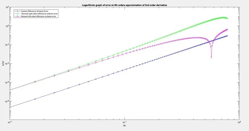

The skewed left and right sided difference schemes both converge it the end ,i.e., their errors are same. But when compared to central difference scheme, they are less accurate.

why a skewed scheme is useful? What can a skewed scheme do that a CD scheme cannot?

The SKEWED SCHEMES are useful when the system dosent have enough data on one side of the selected node. example: Boundary problems.