Week 3.5 - Deriving 4th order approximation of a 2nd order derivative using Taylor Table method
Objective:
To find the fourth-order approximations of a second-order derivative using the central differencing scheme, skewed right-sided difference, and skewed left-sided difference with the help of the Taylor table method, and to compare the analytical derivative with the values that were found for the given function.
SCHEME DERIVATIONS:
CENTRAL DIFFERENCING SCHEME:
To derive a fourth orderapproximation for the second order derivative, we start with this approximation,
making the coefficient of 2nd derivative of x as 1, the equation becomes
The coefficient of the second derivative of x is one, while the coefficients of the other derivatives are zero. The coefficient of the sixth derivative of x is an unknown finite term (which is considered as the error term).
So, the power of delta(x) in the wrong term is 4. This proves that the estimate is on the order of 4.
Taylor's table for a 4th-order approximation of a 2nd-order derivative using the Central Difference Scheme is given as:
Solving the equations, coefficients of each term are obtained and the final equation is as follows
Skewed forward difference scheme:
To derive for an error of order 4, 2nd order derivative can be approximated as
making the coefficient of 2nd derivative of x as 1, the equation becomes
The coefficient of 2nd derivative of x is 1 while that of other derivatives is zero and of 6th derivative of x is an unknown finite term (which is considered as the error term).
Thus, in the error term, the power of delta(x) is 4. This confirms that the approximation is of order 4.
Taylor's table for 4th order approximation of 2nd order derivative using Skewed forward difference scheme is
Solving the equations, coefficients of each term is obtained and the final equation is as follows
Skewed backward difference scheme:
To derive for an error of order 4, 2nd order derivative can be approximated
making the coefficient of 2nd derivative of x as 1, the equation becomes
The coefficient of the second derivative of x is one, while the coefficients of the other derivatives are zero. The coefficient of the sixth derivative of x is an unknown finite term (which is considered as the error term).
So, the power of delta(x) in the wrong term is 4. This proves that the estimate is on the order of 4.
Taylor's table for a 4th-order approximation of a 2nd-order derivative using the skewed forward difference scheme is given as
Solving the equations, coefficients of each term is obtained and the final equation is as follows
To determine the coefficients of the equation, a code was written in Matlab which will solve the algebraic equations.
Main Program:
clear all
close all
clc

%analytical function defination and value assignment
x=pi/3;
dx=linspace(pi/10,pi/1000,100);
f=@(x)(exp(x)*cos(x));
g=@(x)(-2*exp(x)*sin(x));
d2f=g(x);
func=f(x);


%for central difference scheme
%coefficients taken from taylor's table
P = [1 1 1 1 1
    -2 -1 0 1 2
    4/2 1/2 0 1/2 4/2
    -8/6 -1/6 0 1/6 8/6
    16/24 1/24 0 1/24 16/24];


C=[0;0;1;0;0];
%as P*a=C i.e. a=inverse(P)*c(fastest way to getby '\')

cf1=P\C;

%for right skewwd differnce scheme
Q= [1 1 1 1 1 1
    0 1 2 3 4 5
    0 1/2 2 9/2 16/2 25/2
    0 1/6 8/6 27/6 64/6 125/6
    0 1/24 16/24 81/24 256/24 625/24
    0 1/120 32/120 243/120 1024/120 3125/120];
D=[0;0;1;0;0;0];
%as Q*b=s i.e. b=inverse(Q)*s(fastest way to getby '\')

cf2=Q\D;

%for right skewwd differnce scheme
R= [1 1 1 1 1 1
    -5 -4 -3 -2 -1 0
    25/2 16/2 9/2 2 1/2 0
    -125/6 -64/6 -27/6 -8/6 -1/6 0
    625/24 256/24 81/24 16/24 1/24 0
    -3125/120 -1024/120 -243/120 -32/120 -1/120 0];
E=[0;0;1;0;0;0];
%as n*b=s i.e. b=inverse(n)*s(fastest way to getby '\')

cf3=R\E;

%calculating values of derivative using CDS RSDC,LSDC
%defining variable size befor using in loop
central_diff=zeros(1,100);
err_central=zeros(1,100);
right_sdiff=zeros(1,100);
err_right=zeros(1,100);
left_sdiff=zeros(1,100);
err_left=zeros(1,100);

for i=1:length(dx)
    %calculating value and error by central difference scheme
    central_diff(i)=(cf1(1)*f(x-2*dx(i))+cf1(2)*f(x-dx(i))+cf1(3)*f(x)+cf1(4)*f(x+dx(i))+cf1(5)*f(x+2*dx(i)))/(dx(i))^2;
    err_central(i)=abs(central_diff(i)-d2f);

    %calculating value and error by right skewed difference scheme
    right_sdiff(i)=(cf2(1)*f(x)+cf2(2)*f(x+dx(i))+cf2(3)*f(x+2*dx(i))+cf2(4)*f(x+3*dx(i))+cf2(5)*f(x+4*dx(i))+cf2(6)*f(x+5*dx(i)))/(dx(i))^2;
    err_right(i)=abs(right_sdiff(i)-d2f);

    %calculating value and error by left skewed difference scheme
   left_sdiff(i)=(cf3(1)*f(x-5*dx(i))+cf3(2)*f(x-4*dx(i))+cf3(3)*f(x-3*dx(i))+cf3(4)*f(x-2*dx(i))+cf3(5)*f(x-dx(i))+cf3(6)*f(x))/(dx(i))^2;
   err_left(i)=abs(left_sdiff(i)-d2f);

end

%plotting values of derivative
subplot(2,1,1)
hold on
fplot(d2f,'--')
xlim([-0.05 0.35]);
plot(dx,central_diff,'linewidth',2,'color','r');
plot(dx,right_sdiff,'linewidth',2,'color','b');
plot(dx,left_sdiff,'linewidth',2,'color','g');
legend('analytical value at x=pi/3','central diff.','right skewed diff.','left skewed diff.','location','best')
xlabel('Grid siza(dx)');
ylabel('Value');
title('Comparision b\w value of derivative calculated by diff. order of approximation')
hold off

%plotting errors in approximation of derivative
subplot(2,1,2)
loglog(dx,err_central,'linewidth',2,'color','r');
hold on
xlim([.002 0.4]);
loglog(dx,err_right,'linewidth',2,'color','b');
loglog(dx,err_left,'linewidth',2,'color','g');
legend('central diff.','right skewed diff.','left skewed diff.','location','best')
xlabel('Grid siza(dx)');
ylabel('Absolute error');
title('Comparision b/w 4th order approximation method for error in calculating d2f/dx2 ');
Graph:
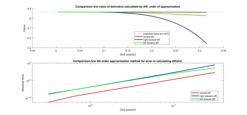
Conclusion:
The figures show that the central difference method is much less likely to be wrong than the skewed methods. Also, the CDS method is better than the skewed method because it has faster convergence rates.
When the time step is small, forward and backward difference methods almost give the same results in terms of error.
CDS can't be used at boundary nodes because forward and backward nodes can't be used at the same time. Depending on the direction of information flow, a forward or backward differencing scheme is used in these situations.