Week 3.5 - Deriving 4th order approximation of a 2nd order derivative using Taylor Table method

Objective :

To derive the  4th order approximations scheme of the second order derivative for

1. Central difference

2. Skewed right sided difference

3. Skewed left sided difference

and also compare these errors with forward and backward difference of first order derivative and  second order approximation .

Deriving the  4th order approximations scheme of the second order derivative 

1. Central difference :

To compute fourth order central difference approximation of second order derivative at a point x we need 4 extra points with the current point i.e; 2 on the left and 2 on the right.

Now, we are considering the hypothesis equation as

                             

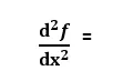
Then calculate the values of a,b,c,d,e ,then you get the required approximation.These values can be found out by using taylors table.

                          

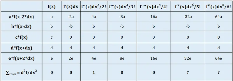
We are trying to compute second order derivative the only terms we should have on the right hand side is f''(x) that means sum of columns in the table for the first 2 columns should be equal to 0 and third column equals to 1 and 4th and 5th column equals to 0 and in the original hypothesis  you have 5 unknowns which means you need only 5 equations to solve the system and remaining what they sum upto we dont know we just ignore higher order terms.

we get ,                  a+b+c+d+e =0               -----(1)

                            -2a-b+0+d+2e=0              -----(2)

                             4a+b+0+d+4e=2            -------(3)

                            -8a-b+0+d+8e=0            ------(4)

                            16a+b+0+d+16e=0          -----(5)

now writing these equations in matrix form A X = B and solving these using matlab by X =inv(A)*B or X =A\B we get the values for a,b,c,d,e

we get,   a=-0.0833;

              b=1.333;

              c=-2.50;

               d=1.333;

            e=-0.0833;

 As we have to equate the coefficients of  dx^2 .f''(u) to 1 ,then our hypothesis equation should be divided by dx^2 to get the required

        

To show that the derived scheme is of  fourth order approximation,we use the formula,

 The order of accuracy P = Number of nodes in the stencil N - order of derivative Q + 1 for symmetric/central schemes

                          p = 5-2+1 =4

 Hence the order of derived scheme is fourth order approximation. we can also verify this by expanding the orginal hypothesis function,

                         

Hence here a =b and b=d the coefficient terms of the fifth derivative get cancelled and =0, then the remaining terms are

                                         

Then divide the equations by dx² on both sides we get, then we can see that in first term of higher order terms, the power of dx will become 4. Then we will ignore the higher order terms i.e., order of 4. Then,

                          

Hence, we can conclude that our derived scheme is of 4^th order accurate.

2. Skewed right sided difference :

To compute fourth order Skewed right sided difference approximation of second order derivative at a point x we need 5 extra points with the current point i.e; 6  on the right.

Now, we are considering the hypothesis equation as

                                  

Then calculate the values of a,b,c,d,e,g ,then you get the required approximation.These values can be found out by using taylors table.

                                  

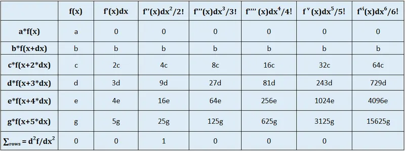
Since we are trying to compute second order derivative  the only terms you should have on the right hand side is f''(x) that means sum of columns in the table for the first 2 columns should be equal to 0 and third column =1 and 4th and 5th and 6th column =0 and in the orginal hypothesis  you have 6 unknowns which means you need only 6 equations to solve the system and remaining what they sum upto we dont know we just ignore higher order terms.

then we get ,                  a+b+c+d+e+g =0                -----(1)

                                0-b+2c+3d+4e+5g=0                -----(2)

                             0+b+4c+9d+16e+25g=2            -------(3)

                          0+b+8c+27d+64e+125g=0             ------(4)

                       0+b+16c+81d+256e+625g=0              -----(5)

                 0+b+32c+243d+1024e+3125g =0           -------(6)

now writing these equations in matrix form A X = B and solving these using matlab by X =inv(A)*B or X =A\B we get the values for a,b,c,d,e,g

we get ,   a= 3.7500;
              b= -12.8333;
             c = 17.8333;
             d = -13.0000;
              e = 5.0833;
              g = -0.8333;

 As we have to equate the coefficients of  dx^2 .f''(u) to 1 ,then our hypothesis equation should be divided by dx^2 to get the required

                    

To show that the derived scheme is of  fourth order approximation,we use the formula,

The order of accuracy P = Number of nodes in the stencil N - order of derivative Q   for one-sided/skewed schemes 

                          p = 6-2 =4

 Hence the order of derived scheme is fourth order approximation.we can also verify this by expanding the orginal hypothesis function,

                                     

Then divide the equations by dx² on both sides we get, then we can see that in first term of higher order terms, the power of dx will become 4. Then we will ignore the higher order terms i.e., order of 4. Then,

                          

Hence, we can conclude that our derived scheme is of 4^th order accurate.

 

3. Skewed left sided difference :

To compute fourth order Skewed left sided difference approximation of second order derivative at a point x we need 5 extra points with the current point i.e; 6 on the left .

Now, we are considering the hypothesis equation as

                          

Then calculate the values of a,b,c,d,e,g ,then you get the required approximation.These values can be found out by using taylors table.

                              

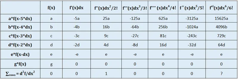
Since we are trying to compute second order derivative the only terms you should have on the right hand side is f''(x) that means sum of columns in the table for the first 2 columns should be equal to 0 and third column =1 and 4th,5th and 6th column =0 and in the orginal hypothesis  you have 6 unknowns which means you need only 6 equations to solve the system and remaining what they sum upto we dont know we just ignore higher order terms.

then we get ,             a+b+c+d+e+g =0                  -----(1)

                            -5a-4b-3c-2d-e+0=0                   -----(2) 

                           25a+16b+9c+4d+e+0=2            -------(3)

                          -125a-64b-27c-8d-e+0=0              ------(4)

                      625a+256b+81c+16d+e+0=0             -----(5)

                    -3125a-1024a-243c-32d-e+0=0          -------(6)

now writing these equations in matrix form A X = B and solving these using matlab by X =inv(A)*B or X =A\B we get the values for a,b,c,d,e

we get ,  a= -0.8333;     
              b= 5.0833;
             c = -13.0000;
             d = 17.8333;
              e = -12.8333;
              g = 3.7500;

 As we have to equate the coefficients of  dx^2 .f''(u) to 1 ,then our hypothesis equation should be divided by dx^2 to get the required,

                    

To show that the derived scheme is of  fourth order approximation,we use the formula,

The order of accuracy P = Number of nodes in the stencil N - order of derivative Q   for one-sided/skewed schemes 

                          p = 6-2 =4

 Hence the order of derived scheme is fourth order approximation.we can also verify this by expanding the orginal hypothesis function,

                                     

Then divide the equations by dx² on both sides we get, then we can see that in first term of higher order terms, the power of dx will become 4. Then we will ignore the higher order terms i.e., order of 4. Then,

                                 

Hence, we can conclude that our derived scheme is of 4^th order accurate.

Now let's compare how the error varies for these schemes when dx is decreased using matlab code.

Matlab Program:

clear all
close all
clc

% defining the function

f=(@(x)exp(x)*cos(x));

% assuming value of x

x=pi;

%range of dx(grid sizing)

dx = linspace(pi/10,pi/10000,50);

%Analytical Derivative of function exp(x)*cos(x) 

Analytical_derivative = -2*exp(x)*sin(x);

% computing the value of 4th order approximations of different schemes of the second order derivative for given function.

for i = 1 :length(dx)
    
   central_difference(i) = (-0.0833*f(x-2*dx(i))+1.3333*f(x-dx(i))-2.5*f(x)+1.3333*f(x+dx(i))-0.0833*f(x+2*dx(i)))/dx(i)^2;
                               
  Skewed_right_sided_difference(i) =(3.75*f(x)-12.8333*f(x+dx(i))+17.8333*f(x+2*dx(i))-13*f(x+3*dx(i))+5.0833*f(x+4*dx(i))-0.8333*f(x+5*dx(i)))/dx(i)^2;
  
   Skewed_left_sided_difference(i) =( -0.8333*f(x-5*dx(i))+5.0833*f(x-4*dx(i))-13*f(x-3*dx(i))+17.8333*f(x-2*dx(i))-12.8333*f(x-dx(i))+3.75*f(x))/dx(i)^2;
   
end

% calculating the absolute error

central_difference_error =abs(Analytical_derivative-central_difference);

Skewed_right_sided_difference_error =abs(Analytical_derivative-Skewed_right_sided_difference);

Skewed_left_sided_difference_error =abs(Analytical_derivative-Skewed_left_sided_difference);

% plotting graph dx vs value of error for derived fourth order schemes

loglog(dx,central_difference_error)
hold on
loglog(dx,Skewed_right_sided_difference_error) 
 hold on
loglog(dx,Skewed_left_sided_difference_error)
title('variation of error as a factor of dx for various fourth order schemes for given function at x=pi')
xlabel('dx(grid size)')
ylabel('value of error')

legend('central difference error','Skewed right sided difference error','Skewed left sided difference error')

Conclusion:

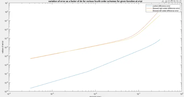
Skewed schemes utilize data from either left or right data points from the point of consideration,whereas central difference scheme us data from both left and right from the  point of consideration.Apparently skewed schemes can be used when direction of flow of a particular entity is known i.e. for example if heat flows over plate from left to right and Skewed right sided scheme is used the solution obtain would contain higher accuracy when compared to CDS. If you want to compute single or higher order derivative at corner node CDS system cannot be used.