Week 3.5 - Deriving 4th order approximation of a 2nd order derivative using Taylor Table method
NUMERICAL APPROXIMATION ANALYSIS -TAYLOR'S TABLE METHOD
AIM:
To write a program that compares the central, Skewed right-sided differencing and skewed left -sided differencing of the fourth order approximations of the second order derivative against the analytical derivative using taylor's table method.
OBJECTIVE:
- To derive the fourth order approximations of the second-order derivative.
- To prove that skewed (Right & Left Sided) and central differencing schemes are of fourth-order accurate.
- To write a program to compute the second derivative of a function f(x) analytically.
- To write a program for the fourth order approximations for the second order derivative against the analytical derivative.
- To determine an error parameter as the absolute difference in numerical and exact derivative.
- To plot the absolute error between the schemes and order of appeoximations.
- To describe a useful of a skewed scheme and also the significane of skewed scheme.
SCHEMES TO DERIVE:
1. Central difference
2. Skewed right-sided difference
3. Skewed left-sided difference
GIVEN DATA'S:
FUNCTION TO COMPUTE:- `f(x)=exp(x)*cos(x)`
@Second Derivative :- `x = pi/3`
Range :- `dx=(pi/30000,pi/4,150)`
INTRODCUTION:
DISCRETIZATION:
Discretization methods are used to divide the region of a continuous function i.e., the real solution to a system of differential equations into a discrete function, where the solution values are defined at each point in space and time. Discretization simply refers to the spacing between each point in solution space and then replace derivatives in the governing equation with difference quotients.
FINITE DIFFERENCE METHOD:
In numerical analysis, finite-difference methods (FDM) are a class of numerical techniques for solving differential equations by approximating derivatives with finite differences. Based on finite differences, it gives the numerical solutions for the values at discrete points in the domain which are known as grid points.
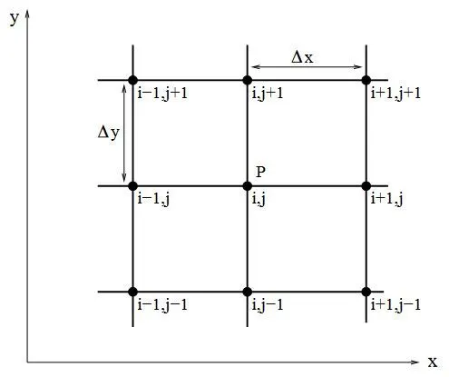
Finite differences method are used to compute approximate derivatives. This is used in numerical analysis in numerical ordinary differential equations and numerical partial differential equations, which gives the numerical solution of ordinary and partial differential equations respectively. The resulting methods are called finite-difference methods. Finite difference representations of derivatives are derived from Taylor series expansions.
DERIVING SECOND ORDER DERIATIVES FOR FOURTH ORDER APPROXIMATION:
1. CENTRAL DIFFERENCING SCHEME:
DETERMINING THE NUMBER OF NODES:-
The order of accuracy, P = 4
Order of derivative, Q = 2
The order of accuracy P = Number of nodes in the stencil N - order of derivative Q+1.
`P = N-Q+1`
Rearranging the equations,
Number of nodes in the stencil, `N=P+Q-1`
Nodes,N = 4+2-1=5
In central differencing scheme the data points are taken from both the sides from 2 nearby data points.
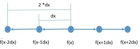
The second Derivative Hypothisis Equation will be,
`(d^2f)/(dx^2)=a*f(x-2dx)+b*f(x-1dx)+c*f(x)+d*f(x+1dx)+e*f(x+2dx)`
DERIVING THE EQUATION FOR CENTRAL DIFFERENCING SCHEME:
`a*f(x-2dx) = a*f(x)-a*2*△x*f'(x)+a*4(△x)^2/2*f''(x)-a*8*(△x)^3/6*f'''(x)+a*16*(△x)^4/24*f''''(x)-`
`-a*32*(△x)^5/120*f'''''(x)`
b*f(x-dx) = `b*f(x)-b*△x*f'(x)+b*(△x)^2/2*f''(x)-b*(△x)^3/6*f'''(x)+b*(△x)^4/24*f''''(x)+...`
`-b*(△x)^5/120*f'''''(x)`
c*f(x) = c* f(x)
d*f(x+dx) = `d*f(x)+d*△x*f'(x)+d*(△x)^2/2*f''(x)+d*(△x)^3/6*f'''(x)+d*(△x)^4/24*f''''(x)+...`
`+d*(△x)^5/120*f'''''(x)`
`e*f(x+2dx) = e*f(x)+e*2*△x*f'(x)+e*4(△x)^2/2*f''(x)+e*8*(△x)^3/6*f'''(x)+...`
`e*16*(△x)^4/24*f''''(x)+e*32*(△x)^5/120*f'''''(x)`
TAYLOR'S TABLE METHOD:
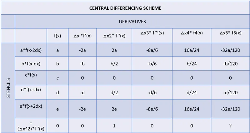
Then, Neglecting the higher order terms and computing 5 unknowns for 5 equations,
`(d^2f)/(dx^2)=a*f(x-2dx)+b*f(x-1dx)+c*f(x)+d*f(x+1dx)+e*f(x+2dx)`
To find the constants a,b,c,d,e, For that Equating the equations,
`a+b+c+d+e= 0;`
`-2a-b+0+d+e=0`
`2a+b/2+0+d/2+2e=1`
`-8a/6-b/6+0+d/6+8e/6=0`
`16a/24+b/24+0+d/24+16e/24=0`
Using Matrix inversion method to solve system of equations, (AX=B):,
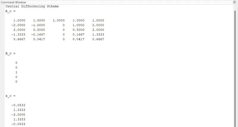
Proof for central differencing schemes are of fourth-order accurate,
Let the equations be,
`(d^2f)/(dx^2)=a*f(x-2dx)+b*f(x-1dx)+c*f(x)+d*f(x+1dx)+e*f(x+2dx)`= `dx^2*f''(x) + dx^6*f^6(x)`
Rewriting the order,
`(d^2f)/(dx^2)= dx^2*f''(x) + dx^6*f^6(x)`
Dividing the equations by `dx^2` on both sides,
`(a*f(x-2dx)+b*f(x-1dx)+c*f(x)+d*f(x+1dx)+e*f(x+2dx))/(dx^2) =f''(x) + 0*dx^4*`
The second-order-accurate difference representation for the derivative can be identified as a fourth-order difference approximation
Here the term,
`(O)*dx^4`
Is called as the the term truncation error of order four O(∆x). The truncation error can be reduced by retaining more terms in the Taylor series expansion of the corresponding derivative and reducing the magnitude of ∆x.
2. SKEWED RIGHT-SIDED DIFFERENCING:
DETERMINING THE NUMBER OF NODES:-
The order of accuracy, P = 4
Order of derivative, Q = 2
The order of accuracy P = Number of nodes in the stencil N - order of derivative Q+1.
`P = N-Q`
Rearranging the equations,
Number of nodes in the stencil, `N=P+Q`
Nodes,N = 4+2=6
In Skewed Right- sided differencing scheme the data points are taken from positive side of data points.
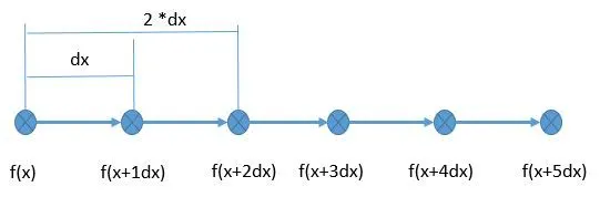
The second Derivative Hypothisis Equation will be,
`(d^2f)/(dx^2)=a*f(x)+b*f(x+dx)+c*f(x+2dx)+d*f(x+3dx)+e*f(x+4dx)+ i*f(x+5dx)`
DERIVING THE EQUATION FOR SKEWED RIGHT-SIDE DIFFERENCING SCHEME:
a*f(x) = a* f(x)
b*f(x+1) = `b*f(x)+b*△x*f'(x)+b*(△x)^2/2*f''(x)+b*(△x)^3/6*f'''(x)+b*(△x)^4/24*f''''(x)+...`
`+b*(△x)^5/120*f'''''(x)`
c*f(x+2) = `c*f(x)+c*2*△x*f'(x)+c*4(△x)^2/2*f''(x)+c*8*(△x)^3/6*f'''(x)+c*16*(△x)^4/24*f''''(x)+...`
`+c*32*(△x)^5/120*f'''''(x)`
`d*f(x+3) = d*f(x)+d*3*△x*f'(x)+d*9*(△x)^2/2*f''(x)+d*27*(△x)^3/6*f'''(x)+..`
`+d*81*(△x)^4/24*f''''(x)+d*243*(△x)^5/120*f'''''(x)`
`e*f(x+4) =e*f(x)+e*4*△x*f'(x)+e*16*(△x)^2/2*f''(x)+e*64*(△x)^3/6*f'''(x)+..`
`+e*256*(△x)^4/24*f''''(x)+e*1024*(△x)^5/120*f'''''(x)`
`i*f(x+5) = i*f(x)+i*5*△x*f'(x)+i*25*(△x)^2/2*f''(x)+i*125*(△x)^3/6*f'''(x)+....`
`+i*625*(△x)^4/24*f''''(x)+i*3125*(△x)^5/120*f'''''(x)`
TAYLOR'S TABLE METHOD:
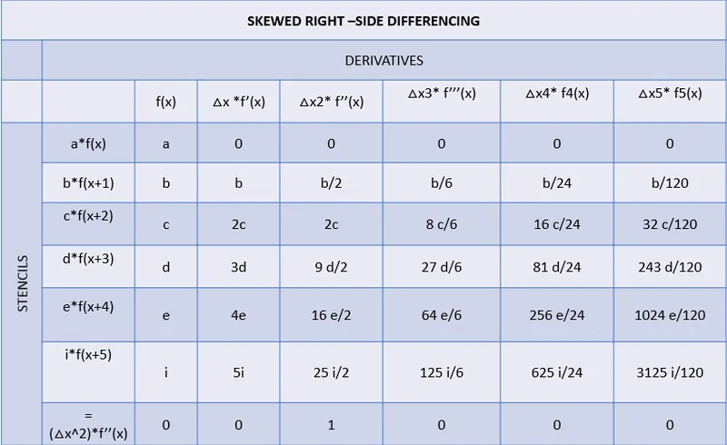
Then,
(△x^2)*f’’(x) = `a*f(x)+b*f(x+dx)+c*f(x+2dx)+d*f(x+3dx)+e*f(x+4dx)+ i*f(x+5dx)`
To find the constants a,b,c,d,e,i, for that Equating the equations,
`a+b+c+d+e+i = 0;`
`0+b+2c+3d+4e+5i=0;`
`0+b/2+2c+9d/2+16e/2+25i/2=1;`
`0+b/6+8c/6+27 d/6+64e/6+125i/6=0;`
`0+b/24+16c/24+81d/24+256e/24+625 i/24=0;`
`0+b/120+32c/120+243 c/120+1024 e/120+3125 i/120=0;`
Using Matrix inversion method to solve system of equations, (AX=B):,
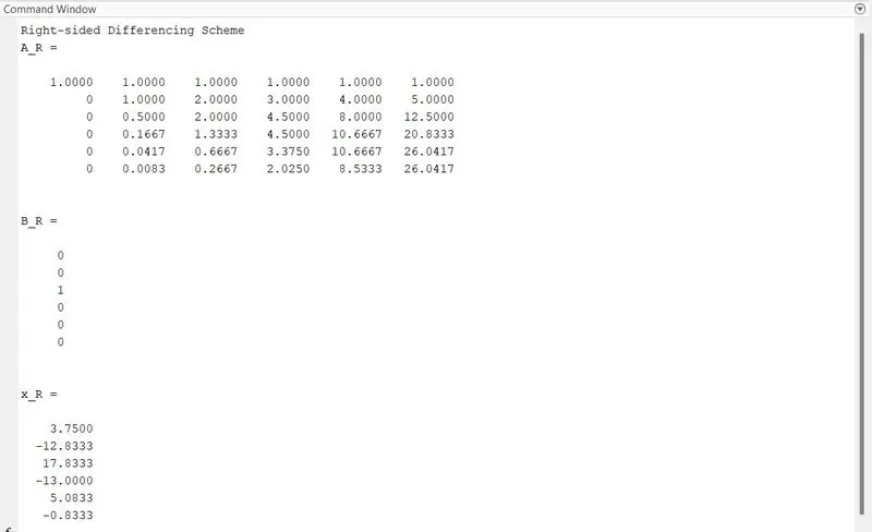
Proof for Right-sided differencing schemes are of fourth-order accurate,
Let the equations be,
`(d^2f)/(dx^2)=a*f(x)+b*f(x+dx)+c*f(x+2dx)+d*f(x+3dx)+e*f(x+4dx)+ i*f(x+5dx)`
Rewriting the order,
`(d^2f)/(dx^2)= dx^2*f''(x) + dx^6*f^6(x)`
Dividing the equations by `dx^2` on both sides,
`a*f(x)+b*f(x+a)+c*f(x+2a)+d*f(x+3a)+e*f(x+4a)+ i*f(x+5a) =f''(x) + 0*dx^4*`
The second-order-accurate difference representation for the derivative can be identified as a fourth-order difference approximation
Here the term,
`(O)*dx^4`
Is called as the the term truncation error of order four O(∆x). The truncation error can be reduced by retaining more terms in the Taylor series expansion of the corresponding derivative and reducing the magnitude of ∆x.
3. SKEWED LEFT-SIDED DIFFERENCING:
DETERMINING THE NUMBER OF NODES:-
The order of accuracy, P = 4
Order of derivative, Q = 2
The order of accuracy P = Number of nodes in the stencil N - order of derivative Q+1.
`P = N-Q`
Rearranging the equations,
Number of nodes in the stencil, `N=P+Q`
Nodes,N = 4+2=6
In Skewed Left- sided differencing scheme the data points are taken from Negative side of data points.
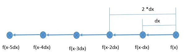
The second Derivative Hypothisis Equation will be,
`(d^2f)/(dx^2)=a*f(x-5dx)+b*f(x-4dx)+c*f(x-3dx)+d*f(x-2dx)+e*f(x-dx)+ i*f(x)`
DERIVING THE EQUATION FOR SKEWED RIGHT-SIDE DIFFERENCING SCHEME:
`a*f(x-5dx) = a*f(x)-a*5*△x*f'(x)+a*25*(△x)^2/2*f''(x)-a*125*(△x)^3/6*f'''(x)+....`
`+a*625*(△x)^4/24*f''''(x)-a*3125*(△x)^5/120*f'''''(x)`
`b*f(x-4dx) =b*f(x)-b*4*△x*f'(x)+b*16*(△x)^2/2*f''(x)-b*64*(△x)^3/6*f'''(x)+..`
`+b*256*(△x)^4/24*f''''(x)-b*1024*(△x)^5/120*f'''''(x)`
`c*f(x-3dx) = c*f(x)-c*3*△x*f'(x)+c*9*(△x)^2/2*f''(x)-c*27*(△x)^3/6*f'''(x)+..`
`+c*81*(△x)^4/24*f''''(x)-c*243*(△x)^5/120*f'''''(x)`
`d*f(x-2dx) = d*f(x)-d*2*△x*f'(x)+d*4(△x)^2/2*f''(x)-d*8*(△x)^3/6*f'''(x)+...`
`+d*16*(△x)^4/24*f''''(x)-d*32*(△x)^5/120*f'''''(x)`
`e*f(x-dx) = e*f(x)-e*△x*f'(x)+e*(△x)^2/2*f''(x)-e*(△x)^3/6*f'''(x)+e*(△x)^4/24*f''''(x)+...`
`-e*(△x)^5/120*f'''''(x)`
`i*f(x) = i* f(x)`
TAYLOR'S TABLE METHOD:
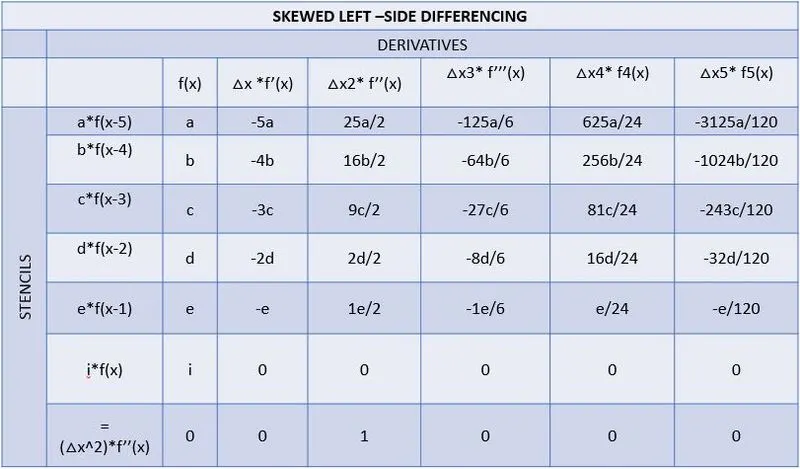
Then,
(△x^2)*f’’(x) = `(d^2f)/(dx^2)=a*f(x-5dx)+b*f(x-4dx)+c*f(x-3dx)+d*f(x-2dx)+e*f(x-dx)+ i*f(x)`
To find the constants a,b,c,d,e,i, for that Equating the equations,
`a+b+c+d+e+i = 0;`
`-5a-4b-3c-2d-e+0=0`
`25a/2+16b/2+9c/2+2d+2e+0=1`
`-125a/6-64b/6-27 c/6-8d/6-e/6+0=0;`
`625 a/24+256e/24+81d/24+16c/24+b/24+0=0;`
`-3125 a/120-1024 b/120-243 c/120-32d/120-e/120+0=0;`
Using Matrix inversion method to solve system of equations, (AX=B):,
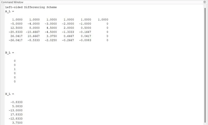
Proof for Left-sided differencing schemes are of fourth-order accurate,
Let the equations be,
`(d^2f)/(dx^2)=a*f(x-5dx)+b*f(x-4dx)+c*f(x-3dx)+d*f(x-2dx)+e*f(x-dx)+ i*f(x)`
Rewriting the order,
`(d^2f)/(dx^2)= dx^2*f''(x) + dx^6*f^6(x)`
Dividing the equations by `dx^2` on both sides,
`a*f(x-5dx)+b*f(x-4dx)+c*f(x-3dx)+d*f(x-2dx)+e*f(x-dx)+ i*f(x) =f''(x) + 0*dx^4*`
The second-order-accurate difference representation for the derivative can be identified as a fourth-order difference approximation
Here the term,
`(O)*dx^4`
Is called as the the term truncation error of order four O(∆x). The truncation error can be reduced by retaining more terms in the Taylor series expansion of the corresponding derivative and reducing the magnitude of ∆x.
ERROR FOR ORDER OF APPROXIMATION:
The error between the approximate solution and the analytical solution is determined by the error that is made by going from a differential operator to a difference operator. This error is called the discretization error or truncation error, the term truncation error reflects the fact that a difference operator can be viewed as a finite part of the infinite taylor's of the differential operator.
Error = abs(Order of Numerical Approximation Derivative - Analytical derivative)
The "abs" returns the Absolute value of the differencr between the numerical and analytical approximation values.
STEPS INVOLVED IN PROGRAMMING:
STEP 1: Defining the function f(x) to compute.
STEP 2: Assigning the inputs for the function f(x).
STEP 3: Solving a function Analytically for the second derivative.
STEP 4: Solving a function numerically by using Central, Skewed Rght and Left schemes .
STEP 5: Solving a Second deriative fourth order approximation using Central differencing scheme.
STEP 6: Solving a Second deriative fourth order approximation using Skewed right sided differencing scheme.
STEP7: Solving a Second deriative fourth order approximation using Skewed Left sided differencing scheme.
STEP 8: Computing the error parameter as the absolute difference in numerical and exact derivative at x = pi/3 & for a range of (dx).
STEP 9: Plotting a absolute error to the range of dx.
STEP 10: Using loglog function to plots x- and y-coordinates using a base-10 logarithmic scale on the x-axis and the y-axis
STEP 11:Using labels and legends the different approximations are identified.
CODING FOR NUMERICAL APPROXIMATION FOR FIRST DERIVATIVE:
FUNCTION FILE:
%% solving a function f(x) Numerically for fourth order approximation of a second derivative,
function [order_of_Approximations]=taylor_eval(x,dx,ct,Analytical_second_derivative)
  for i=1:length(dx)
      % Iterating for a range of dx
        f=exp(x)*cos(x);                       % Given function
        % Right Sided Differencing,
        f_r1=exp(x+dx(i))*cos(x+dx(i));        % (x+1)
        f_r2=exp(x+2*dx(i))*cos(x+2*dx(i));    % (x+2)
        f_r3=exp(x+3*dx(i))*cos(x+3*dx(i));    % (x+3)
        f_r4=exp(x+4*dx(i))*cos(x+4*dx(i));    % (x+4)
        f_r5=exp(x+5*dx(i))*cos(x+5*dx(i));    % (x+5)
        % Left Sided Differencing,
        f_l1=exp(x-dx(i))*cos(x-dx(i));        % (x-1)
        f_l2=exp(x-2*dx(i))*cos(x-2*dx(i));    % (x-2)
        f_l3=exp(x-3*dx(i))*cos(x-3*dx(i));    % (x-3)
        f_l4=exp(x-4*dx(i))*cos(x-4*dx(i));    % (x-4)
        f_l5=exp(x-5*dx(i))*cos(x-5*dx(i));    % (x-5)
    switch ct                              % Switching to (ct) for respective Central,Right & Left Skewed Differencing Aprroximations
        case 1                             % For Central Differencing Approximation
        % Central Differencing Scheme;
        % Determining the co_efficients for central differencing scheme;
        A_c=[1 1 1 1 1;-2 -1 0 1 2;2 1/2 0 1/2 2;-8/6 -1/6 0 1/6 8/6;16/24 1/24 0 1/24 16/24];
        B_c=[0;0;1;0;0];
        x_c=A_c\B_c;
        Central_differ_Aprrox(i)=((x_c(1)*f_l2)+(x_c(2)*f_l1)+(x_c(3)*f)+(x_c(4)*f_r1)+(x_c(5)*f_r2))/(dx(i)^2);
        Error=abs(Central_differ_Aprrox-Analytical_second_derivative);
        case 2                                % For Skewed Right sided Differencing Approximation
        % Skewed Right Sided Diffferencing Scheme;
        % Determining the co-efficients for right sided scheme,
        A_R=[1 1 1 1 1 1;0 1 2 3 4 5;0 1/2 2 9/2 16/2 25/2;0 1/6 8/6 27/6 64/6 125/6;0 1/24 16/24 81/24 256/24 625/24;0 1/120 32/120 243/120 1024/120 3125/120];
        B_R=[0;0;1;0;0;0];
        x_R=A_R\B_R;
        % Skewed Right side differncing approxximaion;
        Skewed_Right_scheme(i)=((x_R(1)*f)+(x_R(2)*f_r1)+(x_R(3)*f_r2)+(x_R(4)*f_r3)+(x_R(5)*f_r4)+(x_R(6)*f_r5))/(dx(i)^2);
        Error=abs(Skewed_Right_scheme-Analytical_second_derivative);
        case 3                                 % For Skewed Left sided Differencing Approximation
        % Skewed Left Sided Diffferencing Scheme;
        % Determining the co-efficients for right sided scheme,
        A_L=[1 1 1 1 1 1;-5 -4 -3 -2 -1 0;25/2 16/2 9/2 2 1/2 0;-125/6 -64/6 -27/6 -8/6 -1/6 0;625/24 256/24 81/24 16/24 1/24 0;-3125/120 -1024/120 -243/120 -32/120 -1/120 0];
        B_L=[0;0;1;0;0;0];
        X_L=A_L\B_L;
        % Skewed left side differncing approxximaion;
        Skewed_Left_scheme(i)=((X_L(1)*f_l5)+(X_L(2)*f_l4)+(X_L(3)*f_l3)+(X_L(4)*f_l2)+(X_L(5)*f_l1)+(X_L(6)*f))/(dx(i)^2);
        Error=abs(Skewed_Left_scheme-Analytical_second_derivative);
    end
  end
order_of_Approximations= (Error);
end
M-CODE:
close all;clc
% Solving second order derivative for fourth order approximation
% By using Central Differencing, Skewed Right side and Skewed Left side differencing
%% Given data's
% Function to compute:- f(x)=exp(x)*cos(x)  @ x=pi/3 for Range dx= pi/30000,pi/4;
%% Solving a function Analytically,
syms y(x)
f(x)=exp(x)*cos(x);
sol=diff(f(x),2);
x=pi/3;
Analytical_second_derivative=double(subs(sol,x));
dx=linspace(pi/30000,pi/4,150);                % Range of Step Size
ct=1:3;                                        % counter for Central Differencing, Skewed Right side and Skewed Left side differencing Approximations
%% Calling a function For Central, Skewed Right and Skewed Left sided Differencing Approximations
   Error_Central_Differ=taylor_eval(x,dx,ct(1),Analytical_second_derivative);
   Error_Skewed_right=taylor_eval(x,dx,ct(2),Analytical_second_derivative);
   Error_Skewed_left=taylor_eval(x,dx,ct(3),Analytical_second_derivative);

%% Plotting Loglog,
figure('Name','COMPARISION OF ORDER OF APPROXIMATIONS-(LogLog Plot)')
loglog(dx,Error_Central_Differ,'LineWidth',1.5)
hold on
loglog(dx,Error_Skewed_right,'LineWidth',1.5)
hold on
loglog(dx,Error_Skewed_left,'LineWidth',1.5)
hold off
title('COMPARISION OF CENTRAL,SKEWED RIGHT & LEFT SIDED DIFFERENCING')
subtitle('Numerical Approximation - Analytical Approximation')
xlabel('Step Size (dx)')
ylabel('Absolute Error')
grid on
legend('Central Differncing Scheme','Skewed Right-Sided Scheme','Skewed Left-Sided Scheme','Location','northwest','box','off')
set(gca,'fontsize',10)
CODING EXPLANATION:
- Defining the function f(x) to solve analytically and numerically for the second derivative.
- Assigning the inputs for the function f(x) @ x=pi/3 for dx range =(pi/30000,pi/4) and dx=(pi/300,pi/4)
- Using linspace command 150 equal number of intervels are assigned as an array for the range dx.
- Then, solving the function f(x) analytically for the second derivative.
- For solving the function f (x) the diff command is used to differentiate analytically for the order of second derivative.
- By using double and subs command the value for X are subsituted in the equation and by solving, determined the analyticall solution for the function f(x).
- The second derivative for the function f(x) are also solved by using product rule.
`-2*exp(x)*sin(x)`
- Creating a function file for solving the central, skewed right sided and skewed left sided differencing schemes based on the inputs passed while calling a function.
- Using "for" loop to iterate each value for the range dx to index.
- Using Switch case statements to solve the central, skewed right sided and skewed left sided differencing schemes @ 1,2,3 respectively based on calling a function.
- Solving a function f(x) Numerically for the central, skewed right sided and skewed left sided differencing schemes.
- Solving a Second deriative fourth order approximation using Central differencing scheme.
- Solving a Second deriative fourth order approximation using Skewed right sided differencing scheme.
- Solving a Second deriative fourth order approximation using Skewed left sided differencing scheme.
- Determining the absolute error by differencing the Numerical approximation values and Analyticall approximation values.
- The errors are determined for the central, skewed right sided and skewed left sided differencing schemes.
- Plotting the error parameter as the absolute difference in numerical and exact derivative at x = pi/3 and also for dx range =(pi/30000,pi/4,150) and dx=(pi/300,pi/4,150)
- Using loglog function to plots x- and y-coordinates using a base-10 logarithmic scale on the x-axis and the y-axis.
- By using legend the Absolute error for the central, skewed right sided and skewed left sided differencing schemes.
PLOTTING:
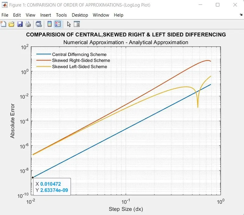
For Range dx=(pi/300,pi/4,150)
For Range dx=(pi/30000,pi/4,150)
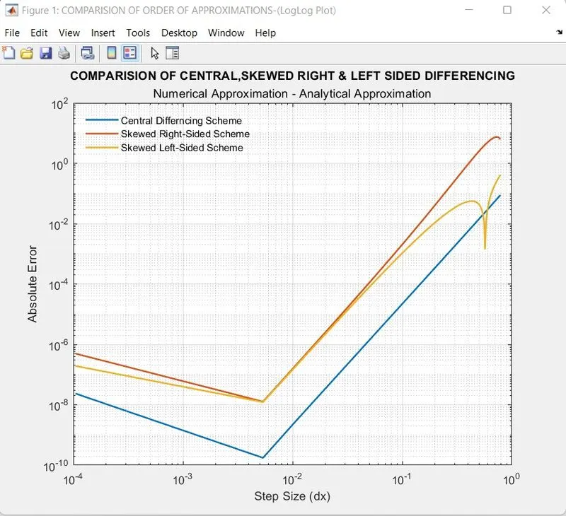
- The plotting describes the relation of order of approximations step size (dx) Range to the error derivative for the respective central, skewed right sided and skewed left sided differencing schemes for the second derivative for numerically and analytically.
- The first plot for Range dx=(pi/300,pi/4,150) the error for the central scheme is acurate solutions compared to skewed right and left differencing schemes.In the second plot for Range dx=(pi/30000,pi/4,150) also the error for the central scheme is accurate solutions compared to skewed right and left differencing schemes.
Comparing to plot 1 and plot 2, When increasing the range of dx (step size) from 10 ^-2 to 10^-4,the error also starts increasing. - The total numerical error is the summation of the truncation and round-off errors. In general, the way to minimize round-off errors is to increase the number of significant figures used in the calculation. Round-off error increases due to subtractive cancellation and as the number of calculations in an analysis grows.
- From the error and the plotting shows that for the central differncing scheme the error value will be accurate then compared to skewed right and left differencing schemes.
SKEWED SCHEME USEFUL AND SIGNIFICANECE OF SKEWED SCHEME OVER CENTRAL DIFFERENCING:
- In Central Differencing scheme the data points are taken from both positive and negative sides from the central node points. If the data values are equally spaced, the central difference is an average of the forward and backward differences.
- In Skewed schemes the data points are selected from one direction of the data node's ie; from positive side called as skewed right sided differencing scheme or from negative side called as skewed left sided differencing scheme.
- Also, in central differencing, from the central node the data points are approximated to the right and left so the error for the order of approximations are accurate and lesser.
- A function is depend on the domain's bondaries. When we are trying to solve the boundaries in the domain in that some cases the central differencing scheme is not usefull. For that the skewed schemes are used to approximate the functions by differencing the data points from right sided or left sided differencing approximations.
M-CODE LINK:
CONCLUSION:
- The fourth order approximations of the second-order derivative for central, skewed right side and skewed left side differencing are been derived.
- The skewed and central differencing schemes are order of fourth-order accurate are proffed.
- The program to compute the second derivative of a function f(x) are derived analytically.
- The program that compares the fourth order approximations for the second order derivative against the analytical derivative for the range of dx are performed and analysed.
- The error parameter as the absolute difference in numerical and exact derivative are computed.
- The plot showing the central, skewed right side and skewed left side differencing of the second derivative against the analytical derivative error are plotted and errors are computed using loglog function plot.