Week 3.5 - Deriving 4th order approximation of a 2nd order derivative using Taylor Table method

To derive the fourth order approximation of the second order derivative :

1.central difference

2.Skewed right-sided difference

3.Skewed left-sided difference

After deriving these schemes, prove that your skewed schemes are fourth-order accurate

write a program in Matlab to evaluate the second-order derivative of the analytical function exp(x)*cos(x) and compare it with the 3 numerical approximations that you have derived.

HINT :

i) The order of accuracy P = Number of nodes in the stencil N - order of derivative Q + 1 for symmetric/central schemes

ii) The order of accuracy P = Number of nodes in the stencil N - order of derivative Q for one-sided/skewed schemes

iii) Solve the system of equations using the matrix inversion method in Matlab to obtain the taylor table coefficients and use them directly in the numerical approximation statements to avoid input errors.

1. CENTRAL DIFFERENCING :

Deriving the central differencing for the fourth order approximation of the second order deriative of a function using Taylor's table method

To find central differencinng we need to find the number of nodes required to evaluate the second order accurate

Number of nodes N = P+Q-1

Where,

P = Order of derivative

Q = order of approximation

For fourth order approximation of the second order derivative,number of nodes required to derive central differencing is

N = 2+4-1 = 5

The second order derivative is expressed as

`trianglex^2 f''(x) = af(i-2)+bf(i-1)+cf(i)+df(i+1)+ef(i+2)`

Evaluating the each term of the hypothesis using Taylor's series

`af(i-2) = a[f(i)-2trianglex/1! f'(i) + (2trianglex)^2/2 ! f''(i)-(2trianglex)^3/3! f'''(i)+(2trianglex)^4/4!+.......`

`bf(i-1) = b[f(i)-trianglex/1! f'(x) + (trianglex)^2/2! f''(i)-(trianglex)^3/3! f'''(i)+(trianglex)^4/4! f''''(i)+....`

`cf(i) = cf(i)`

`df(i+1) = d[f(i)+trianglex/1! f'(i)+(trianglex)^2/2! f''(i)+(trianglex)^3/3! f'''(i) +(trianglex)^4/4! f''''(i)`

`ef(i+2) = e[f(i) + 2trianglex/1! f'(i)+(2trianglex)^2/2! f''(i)+(2trianglex)^3/3! f'''(i) +(2trianglex)^4/41 f''''(i)`

Taylor's table

`trianglex^2 partial^2f/partialx^2 f(i) trianglexf'(i) trianglex^2f''(i) trianglex^3f'''(i) trianglex^4f''''(i)`

af(i-2) a -2a 4a/2 -8a/6 16a/24

bf(i-1) b -b b/2 -b/6 b/24

cf(i) c 0 0 0 0

df(i+1) d d d/2 d/6 d/24

ef(i+2) e 2e 4e/2 8e/6 16e/24

Evaluation for second order derivattive

0 0 1 0 0

With the help of taylor table we can find the values of the coefficients by forming the equations

1. a+b+c+d+e = 0

2.-2a-b+d+2e = 0

3.4a/2+b/2+d/2+4e/2 = 1

4.-8a/6-b/6+d/6+8e/6 = 0

5.16a/24 +b/24+d/24+16e/24 = 0

COMMAND WINDOW :

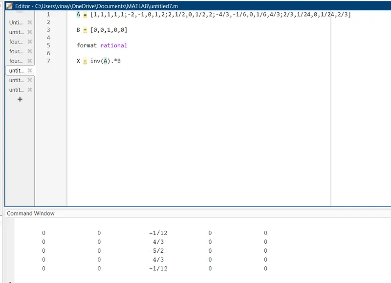
on solving these equations we get the values of the coefficients and these values of the coefficients are used in the equation 1 for derivving the second order derivative for the fourth order aapproximation of the function for central differencing.

2.SKEWED-RIGHT SIDED DIFFERENCE :

In this method same procedure is followed as followed in the SKEWED RIGHT SIDED differencing

The number of nodes required,

N = P+Q

Where,

P = Order of derivative

Q = order of approximation

For fourth order approximation of the second order derivative,number of nodes required to derive skewed right-sided difference is

N = 2+4 = 6.

The second order derivative is expressed as

`trianglex^2 f''(x) = af(i)+bf(i+1)+cf(i+2)+df(i+3)+ef(i+4)+gf(i+5)+.......`

Evaluating the each term of the hypothesis using Taylor's series

`af(i) = af(i)`

`bf(i+1) = b[f(i)+trianglex/1! f'(x) + (trianglex)^2/2! f''(i)+(trianglex)^3/3! f'''(i)+(trianglex)^4/4! f''''(i)+....`

`cf(i+2) = c[f(i)+2trianglex/1! f'(i) + (2trianglex)^2/2! f''(i) +(2trianglex)^3/3! f'''(i) +(2trianglex)^4/4! f''''(i)+......`

`df(i+3) = d[f(i)+3trianglex/1! f'(i)+(3trianglex)^2/2! f''(i)+(3trianglex)^3/3! f'''(i) +(3trianglex)^4/4! f''''(i)`

`ef(i+4) = d[f(i)+4trianglex/1! f'(i)+(4trianglex)^2/2! f''(i)+(4trianglex)^3/3! f'''(i) +(4trianglex)^4/4! f''''(i)`

`gf(i+5) = e[f(i) + 5trianglex/1! f'(i)+(5trianglex)^2/2! f''(i)+(5trianglex)^3/3! f'''(i) +(5trianglex)^4/41 f''''(i)`

Generating taylor's table:

`trianglex^2 partial^2f/partialx^2 f(i) trianglexf'(i) trianglex^2f''(i) trianglex^3f'''(i) trianglex^4f''''(i) trianglex^5f'''''(i)`

af(i) a 0 0 0 0 0

bf(i+1) b b b/2 b/6 b/24 b/120

cf(i+2) c 2c 4c/2 8c/6 16c/24 32c/120

df(i+3) d 3d 9d/2 27d/6 81d/24 243d/120

ef(i+4) e 4e 16e/2 64e/6 256e/24 1024e/120

gf(i+5) g 5g 25g/2 125g/6 625g/24 3125g/120

Evaluation for second order derivattive

0 0 1 0 0

With the help of taylor table we can find the values of the coefficients by forming the equations,

1. a+b+c+d+e+g = 0

2.b+2c+3d+4e+5g = 0

3.b/2 +4c/2 +9d/2 +16e/2+25g/2 = 1

4.b/6 +8c/6 +27d/6 +64e/6 +125g/6 = 0

5.b/24 +16c/24 +81d/24 +256e/24 +625g/24 = 0

6.b/120 +32c/120 +243d/120 +1024e/120 +3125g/120 = 0

COMMAND WINDOW :

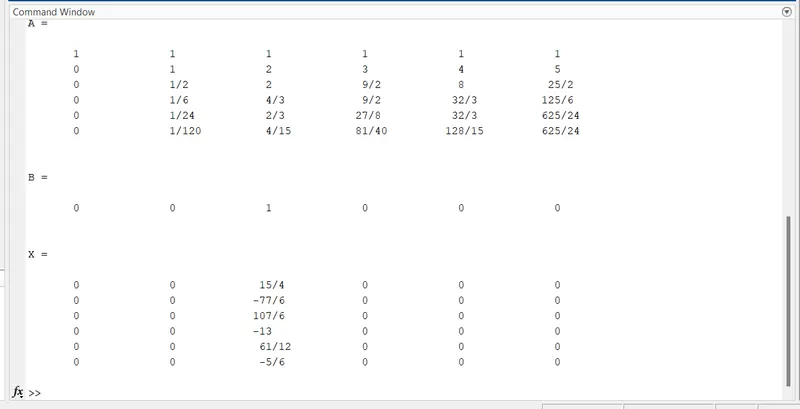
on solving these equations we get the values of the coefficients and these values of the coefficients are used in the equation 2 for deriving the second order derivative for the fourth order aapproximation of the function for skewed right sided differencing.

3.SKEWED LEFT-SIDED DIFFERENCE :

In this method same procedure is followed as followed in the Skewed left-sided differencing

The number of nodes required,

N = P+Q

Where,

P = Order of derivative

Q = order of approximation

For fourth order approximation of the second order derivative,number of nodes required to derive skewed left-sided difference is

N = 2+4 = 6.

`af(i-5) = a[f(i) -5trianglex/1! f'(i)+(5trianglex)^2/2! f''(i)-(5trianglex)^3/3! f'''(i) +(5trianglex)^4/41 f''''(i)`

`bf(i-4) = b[f(i)-4trianglex/1! f'(i)+(4trianglex)^2/2! f''(i)-(4trianglex)^3/3! f'''(i) +(4trianglex)^4/4! f''''(i)`

`cf(i-3) = d[f(i)-3trianglex/1! f'(i)+(3trianglex)^2/2! f''(i)-(3trianglex)^3/3! f'''(i) +(3trianglex)^4/4! f''''(i)`

`df(i-2) = d[f(i)-2trianglex/1! f'(i) + (2trianglex)^2/2! f''(i) -(2trianglex)^3/3! f'''(i) +(2trianglex)^4/4! f''''(i)+......`

`ef(i-1) = b[f(i)-trianglex/1! f'(x) + (trianglex)^2/2! f''(i)-(trianglex)^3/3! f'''(i)+(trianglex)^4/4! f''''(i)+....`

`gf(i) = gf(i)`

Generating taylor's table :

af(i-5) a -5a 25a/2 -125a/6 625a/24 -3125a/120

bf(i-4) b -4b 16b/2 - 64b/6 256b/24 -1024b/120

cf(i-3) c -3c 9c/2 -27c/6 81c/24 -243c/120

df(i-2) d -2d 4d/2 -8d/6 16d/24 -32d/120

ef(i-1) e -e e/2 -e/6 e/24 -e/120

gf(i) g 0 0 0 0 0

1. a+b+c+d+e+g = 0

2. -5a-4b-3c-2d-e = 0

3.25a/2+16b/2+9c/2+4d/2+e/2 = 1

4.-125a/6-64b/6-27c/6-8d/6-e/6 = 0

5.625a/24+256d/24+81c/24+16d/24+e/24 = 0

6.-3125a/120-1024b/120-243c/120-32d/120-e/120 = 0

COMMAND WINDOW :

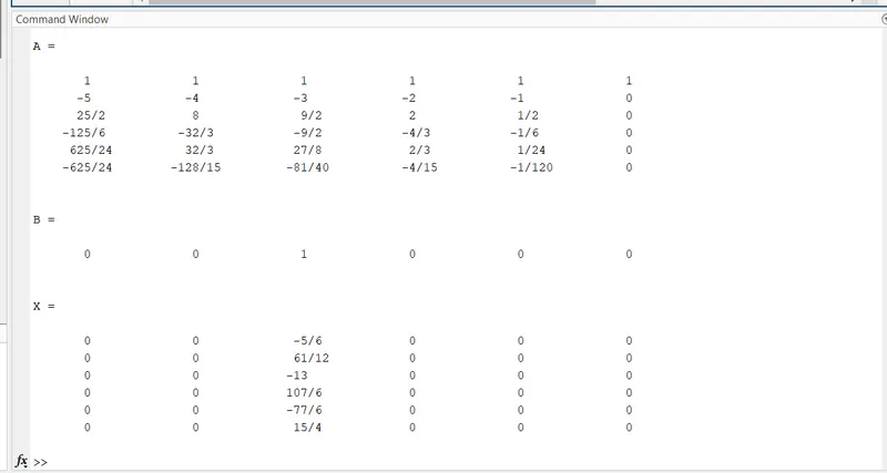
on solving these equations we get the values of the coefficients and these values of the coefficients are used in the equation 3 for deriving the second order derivative for the fourth order aapproximation of the function for skewed left sided differencing.

MAIN PROGRAM :

clear all
close all
clc

% value of x
x = pi/3;

% range of dx

%dx = linspace(pi/4000,pi/40,20);
dx = linspace(pi/40,pi/4000,20);

% creating for loop for the problem

for i = 1:length(dx)

    central_differencing(i) = fourth_order_central_differencing(x,dx(i));
    
    skewed_right_sided_differencing(i) = fourth_order_skewed_right_sided_differencing(x,dx(i));

    skewed_left_sided_differencing(i) = fourth_order_skewed_left_sided_differencing(x,dx(i));

end

% plotting
figure(1)
loglog(dx,central_differencing,'color','b')
hold on
loglog(dx,skewed_right_sided_differencing,'color','r')
hold on
loglog(dx,skewed_left_sided_differencing,'color','g')
xlabel('Range of dx')
ylabel('Truncation error')
title('Range of dx vs Truncation error')
legend('central differencing','skewed right','skewed left')

The above given program is the main program used for calculating fourth order approximation of the second order derivative.

Three functions are created for the main program to get the accurate results.

By using the accurate results ,we get a plot .

WORKSPACE :

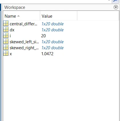
The workspace stores the output values of the program.It is used as a storage for program values..

FUNCTION FOR CENTRAL DIFFERENCING :

function Error_central_differencing = fourth_order_central_differencing(x,dx)


% analytic derivative  = exp(x)*cos(x)
%f''(x) = -2*exp(x)*sin(x)

analytic_derivative = -2*exp(x)*sin(x);

%numerical derivative

% central differencing
central_differencing = (((-1/12)*((exp(x-(2*dx)))*(cos(x-(2*dx)))))+((4/3)*((exp(x-dx))*(cos(x-dx))))-((-5/2)*((exp(x))*(cos(x))))+((4/3)*((exp(x+dx))*(cos(x+dx))))-((-1/12)*((exp(x+(2*dx)))*(cos(x+(2*dx))))))/(dx^2);

Error_central_differencing = abs(central_differencing-analytic_derivative);
end​

Function created for central differencing by using the coefficients obtained by using the taylors table.

FUNCTION FOR SKEWED RIGHT SIDED DIFFERENCING :

function Error_skewed_right_sided_differencing = fourth_order_skewed_right_sided_differencing(x,dx)


% analytic derivative  = exp(x)*cos(x)
%f''(x) = -2*exp(x)*sin(x)

analytic_derivative = -2*exp(x)*sin(x);

%numerical derivative

skewed_right_sided_differencing = (((15/4)*((exp(x))*(cos(x))))-((-77/6)*((exp(x+dx))*(cos(x+dx))))+((107/6)*((exp(x+(2*dx)))*(cos(x+(2*dx)))))-((-13)*((exp(x+(3*dx)))*(cos(x+(3*dx)))))+((61/12)*((exp(x+(4*dx)))))-((-5/6)*((exp(x+(5*dx)))*(cos(x+(5*dx))))))/(dx^2);

%error
Error_skewed_right_sided_differencing = abs(skewed_right_sided_differencing-analytic_derivative);

end

Function created for skewed right sided differencing by using the coefficients obtained by using the taylors table.

FUNCTION FOR SKEWED LEFT SIDED DIFFERENCING :

function Error_skewed_left_sided_differencing = fourth_order_skewed_left_sided_differencing(x,dx)


% analytic derivative  = exp(x)*cos(x)
%f''(x) = -2*exp(x)*sin(x)

analytic_derivative = -2*exp(x)*sin(x);

%numerical derivative

skewed_left_sided_differencing = (((-5/6)*((exp(x-(5*dx)))*(cos(x-(5*dx)))))+((61/12)*((exp(x-(4*dx)))*(cos(x-(4*dx)))))-((-13)*((exp(x-(3*dx)))*(cos(x-(3*dx)))))+((107/6)*((exp(x-(2*dx))))*(cos(x-(2*dx)))))-((-77/6)*((exp(x-dx))*(cos(x-dx))))+((15/4)*((exp(x))*(cos(x))))/(dx^2);

%error

Error_skewed_left_sided_differencing = abs(skewed_left_sided_differencing-analytic_derivative);

end

Function created for skewed left sided differencing by using the coefficients obtained by using the taylors table.

PLOT COMPARES ABSOLUTE ERRORS :

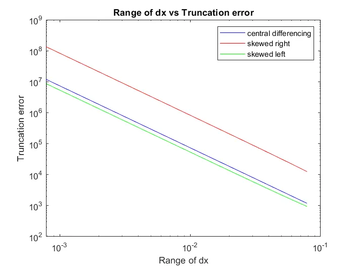
From the above plot we can conclude that central differencing has less errors compared to two others schemes .Because it uses the information form both the sides of the stencils.

In right sided differencing ,information is used from one point interest and it gives less accurate results.

In left sided differencing also ,information is used from one point interest and it gives less accurate results.

xlabel represnts range of dx.

ylabel represnts truncation.

WHY A SKEWED SCHEME IS USEFUL ?

The system which doesn't contain sufficient information on both sides of the point of interest.In such cases we cannot use central differencing scheme so skewed scheme is useful in such cases.

WHAT CAN A SKEWED SCHEME DO THAT A CD SCHEME CANNOT DO ?

CENTRAL DIFFERENCING cannot be employed at the boundary nodes due to unavailability of the right and left nodes at the same time.In such cases the skewed differencing scheme is used.