Week 3.5 - Deriving 4th order approximation of a 2nd order derivative using Taylor Table method

Aim : To derive Fourth order approximation of second order derivative using Taylors Table Method

Objective :

1. to understand taylors table method of discreatization

2 to build thorough understanding of Matlab code for discreatizing fourth order derivative

3 Analyze errors occurance in fourth order left side ,right side skewed and centrel methods of approximation

Theory :

i) The order of accuracy (p) = Number of nodes in the stencil (N) - order of derivative (Q) + 1 for symmetric/central schemes

ii) The order of accuracy (P )= Number of nodes in the stencil (N) - order of derivative (Q) for one-sided/skewed schemes

for fourth order scheme P =4 we have order of derivative =2

for centrel/symmetric schemes, nodes = 5

P =N-Q +1

4 = 5-2 +1 = 4 ,

for one sided /skewed schemes, nodes = 6

P =N-Q

4 = 6-2=4

EQUATION USED

`f(x) = exp(x)*cos(x)`

input

x =pi/3

Question1. why a skewed scheme is useful?

skewed scheme is usefull when both sides nodes are not avalaible during solving a problem it can still solve the equation by taking one sided nodes inputs

Question2. What can a skewed scheme do that a CD scheme cannot?

CD scheme is not usefull near boundary as boundary doesnt have any node so in this case skewed scheme is usefull

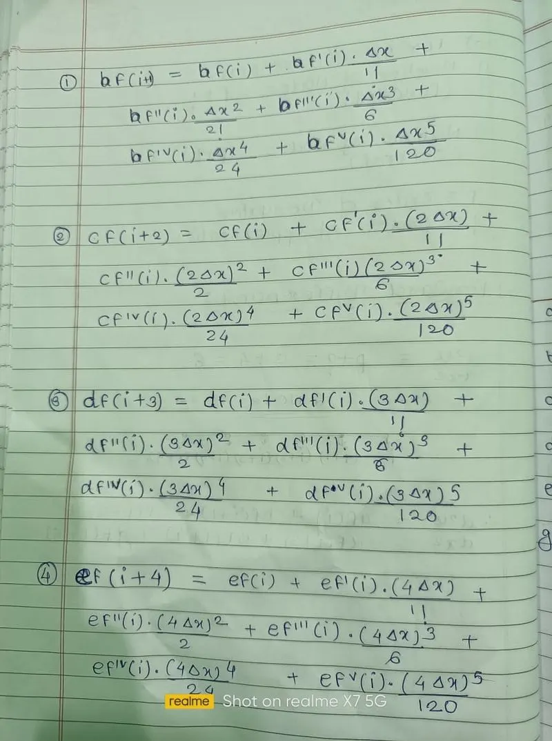
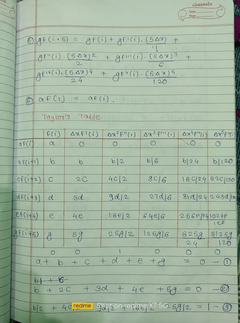
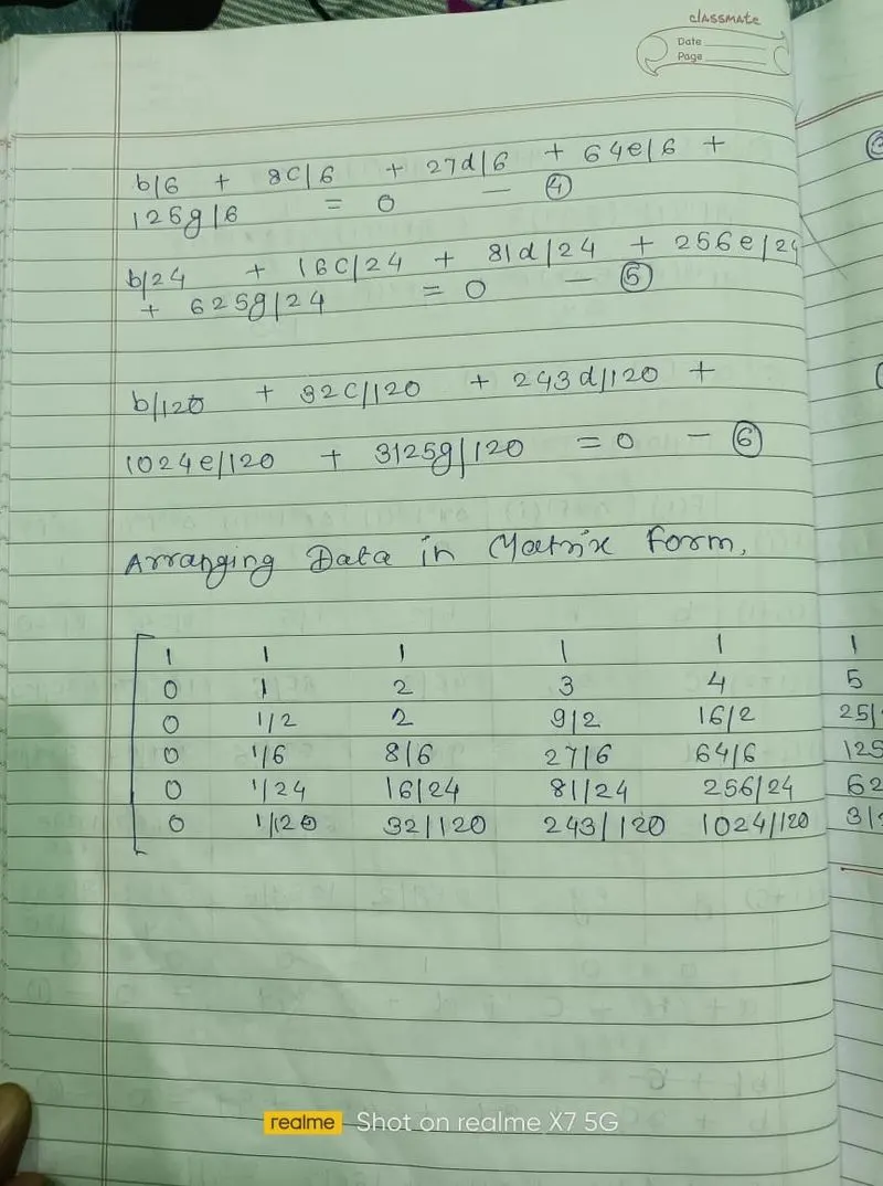
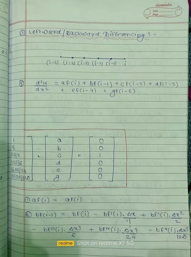
Derivation

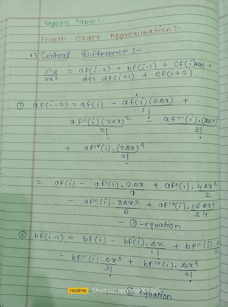
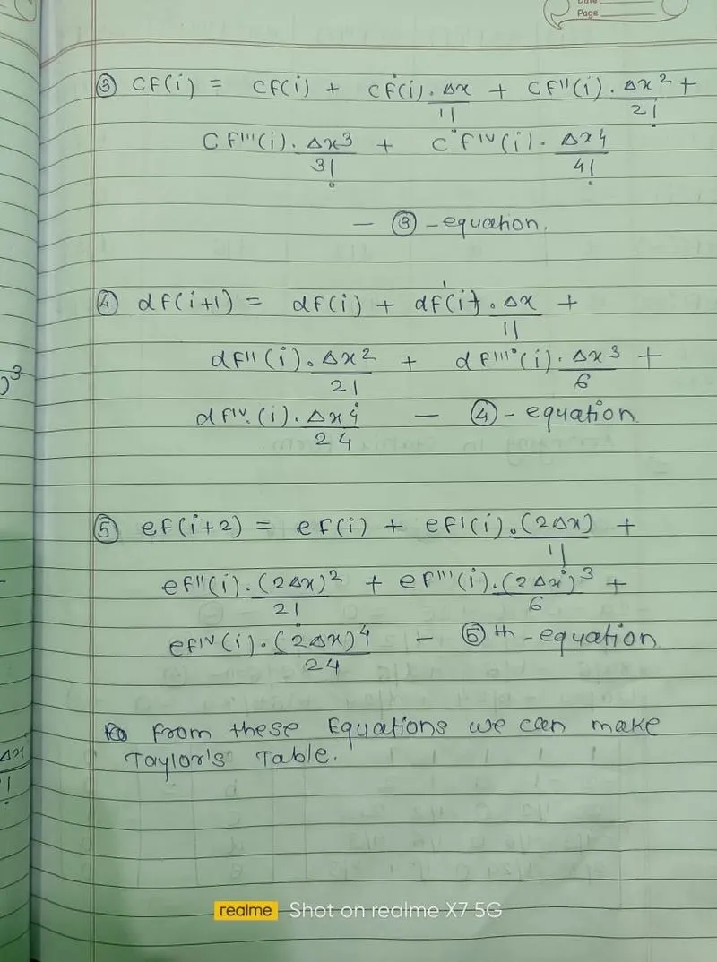
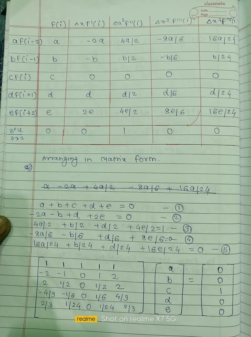
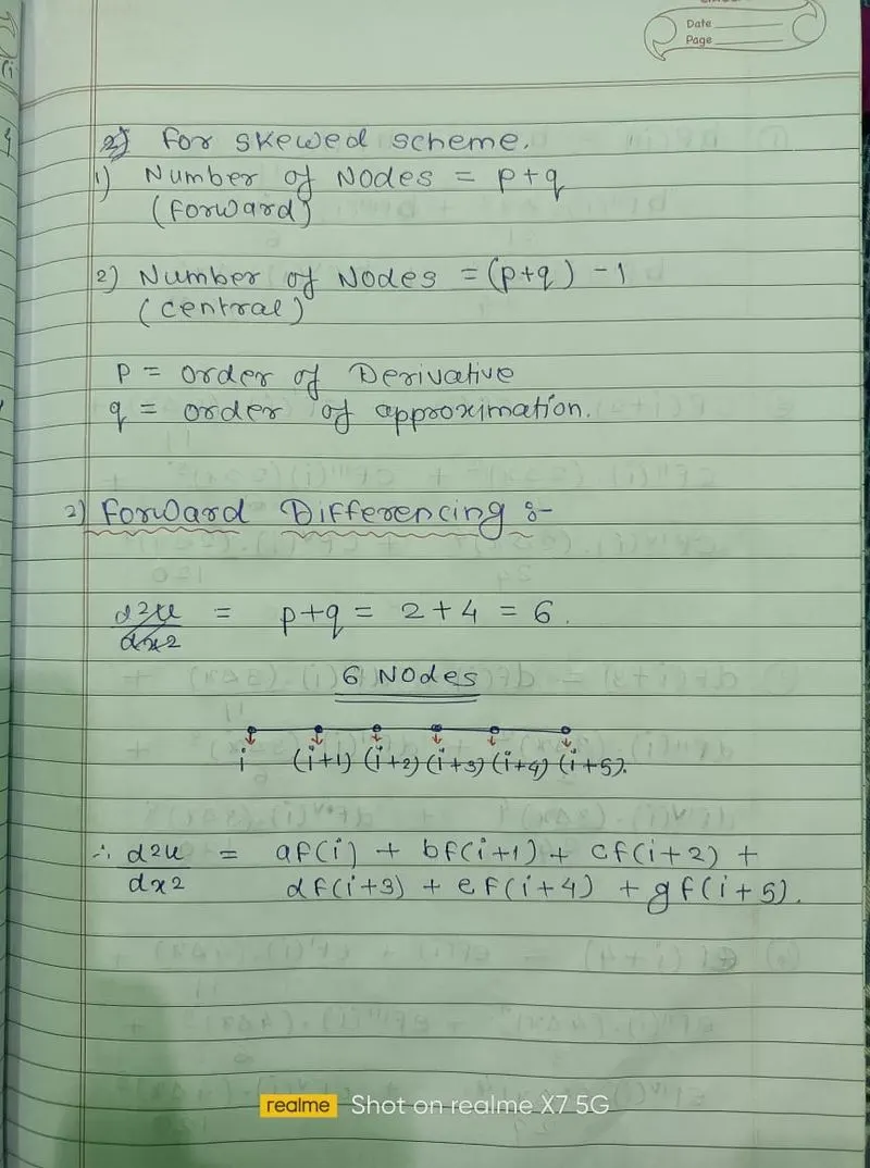
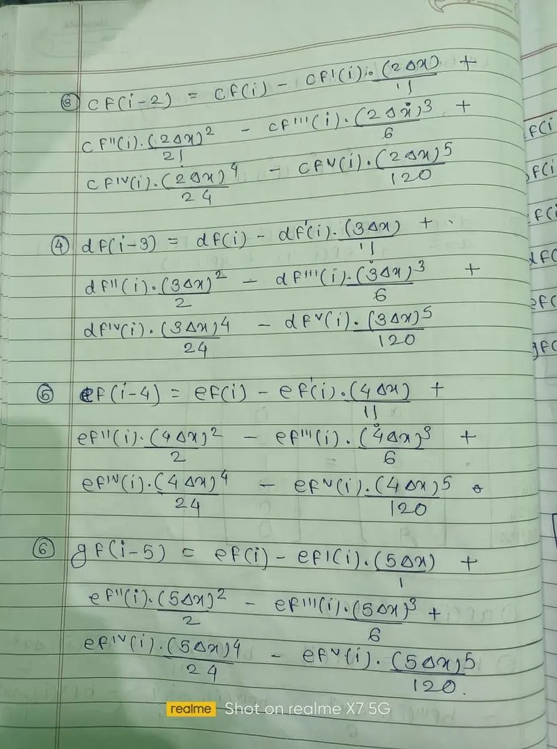
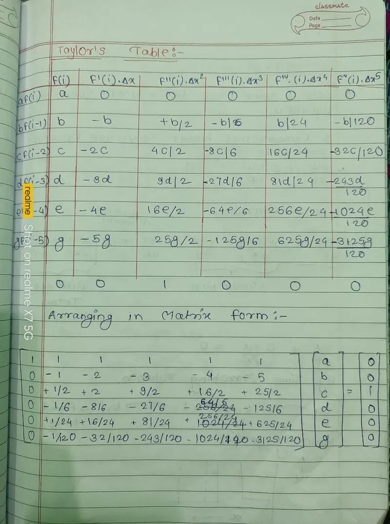
MAIN PROGRAMME :

close all 
clear all
clc
%% Inputs 
x = pi/3;
dx = linspace(pi/400,pi/4,200);
%% Analytical Solution

f_x = exp(x)*cos(x);
f_1dash = exp(x)*(cos(x)-sin(x)); % first derivative 
for i =1:length(dx)
f_2dash(i) = f_1dash - exp(x)*(sin(x) + cos(x)); % second derivative 
end

%% Numerical Solution 
% Centrel differencing 

[f_2dash_cd] = Central_diff(x,dx);
for i =1:length(dx)
error_cd(i) = abs(f_2dash_cd(i)-f_2dash(i));
end 
% Forward diffferencing 
[f_2dash_fd] = forward_diff(x,dx);
for i= 1:length(dx)
error_fd(i) = abs(f_2dash_fd(i)-f_2dash(i));
end
% Backward differencing 
[f_2dash_bd] = backward_diff(x,dx);
for i = 1:length(dx)
error_bd(i) = abs(f_2dash_bd(i)-f_2dash(i));
end
%% plotting 
loglog(dx,error_cd,'color','b','marker','d');
hold on 
loglog(dx,error_fd,'color','k','marker','s');
hold on 
loglog(dx,error_bd,'color','r','marker','o');
grid on 
legend('centrel diffferencing','forward differencing','backward differencing')
title('4th order differencing error');
xlabel('dx');
ylabel('Absolute Error');

Function for Centrel Differencing

function [f_2dash_cd] = Central_diff(x,dx);
% coefficients calculation 
format rational
A = [1 1 1 1 1;-2 -1 0 1 2;2 1/2 0 1/2 2;-4/3 -1/6 0 1/6 4/3; 2/3 1/24 0 1/24 2/3];
B = [0 ; 0 ; 1 ; 0 ; 0];
X = inv(A)*B
a = X(1)
b = X(2)
c = X(3)
d = X(4)
e = X(5)
for i = 1:length(dx)
term1(i) = exp(x-(2.*dx(i))).*cos(x-(2.*dx(i)));
term2(i) = exp(x-dx(i)).*cos(x-dx(i));
term3(i) = exp(x).*cos(x);
term4(i) = exp(x+dx(i)).*cos(x+dx(i));
term5(i) = exp(x+(2.*dx(i))).*cos(x+(2.*dx(i)));
f_2dash_cd(i) = (a.*term1(i) + b.*term2(i) + c.*term3(i) + d.*term4(i) + e.*term5(i))./(dx(i).^2) ;
end
end

Function For Forward/Right side differencing :

function [f_2dash_fd] = forward_diff(x,dx);
% coefficient calculation 
format rational 
A = [1 1 1 1 1 1;0 1 2 3 4 5;0 1/2 2 9/2 16/2 25/2; 0 1/6 8/6 27/6 64/6 125/6; 0 1/24 16/24 81/24 256/24 625/24; 0 1/120 32/120 243/120 1024/120 3125/120 ]
B = [0;0;1;0;0;0];
X = inv(A)*B
a = X(1)
b = X(2)
c = X(3)
d = X(4)
e = X(5)
g = X(6)

for i =1:length(dx)
term1(i) = a.*(exp(x).*cos(x));
term2(i) = b.*(exp(x+dx(i)).*cos(x+dx(i)));
term3(i) = c.*(exp(x+(2.*dx(i))).*cos(x+(2.*dx(i))));
term4(i) = d.*(exp(x+(3.*dx(i))).*cos(x+(3.*dx(i))));
term5(i) = e.*(exp(x+(4.*dx(i))).*cos(x+(4.*dx(i))));
term6(i) = g.*(exp(x+(5.*dx(i))).*cos(x+(5.*dx(i))));
f_2dash_fd(i) = (term1(i) + term2(i) + term3(i) + term4(i) + term5(i) + term6(i))./(dx(i).^2) ;
end 
end

Function for Backward/Leftward Differencing :

function [f_2dash_bd] = backward_diff(x,dx);
% coefficient calculation 
format rational 
A = [1 1 1 1 1 1;0 -1 -2 -3 -4 -5;0 1/2 2 9/2 16/2 25/2; 0 -1/6 -8/6 -27/6 -64/6 -125/6; 0 1/24 16/24 81/24 256/24 625/24; 0 -1/120 -32/120 -243/120 -1024/120 -3125/120 ]
B = [0;0;1;0;0;0];
X = inv(A)*B
a = X(1)
b = X(2)
c = X(3)
d = X(4)
e = X(5)
g = X(6)
for i =1:length(dx)
term1(i) = a.*(exp(x).*cos(x));
term2(i) =  b.*(exp(x-dx(i)).*cos(x-dx(i)));
term3(i) = c.*(exp(x-(2.*dx(i))).*cos(x-(2.*dx(i))));
term4(i) = d.*(exp(x-(3.*dx(i))).*cos(x-(3.*dx(i))));
term5(i) = e.*(exp(x-(4.*dx(i))).*cos(x-(4.*dx(i))));
term6(i) = g.*(exp(x-(5.*dx(i))).*cos(x-(5.*dx(i))));
f_2dash_bd(i) = (term1(i) + term2(i) + term3(i) + term4(i) + term5(i) + term6(i))./(dx(i).^2) ;
end
end

EXPLANATION OF CODE :

1. i have calculated analytical solution of given derivative

2. derived fourth order approximation using taylors table and found values of coefficients by hand calculation

3. form the matrix for solving linear equation and found coefficients value using matlab

4. compared these value with written calculation

5. used function command to form function of seperate method

6. coupled this equation in main programme and using this i calculated Absolute errors

7. Plotted this results and analyze this results

Results :

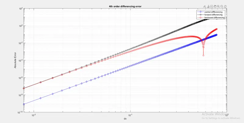
Explanation of plot

1.we can see that when value of dx is less error tends to lesser and lesser having linear variation

2.centrel differencing method have least error compare to other methods